Cerebral aneurysm fluid-solid interaction: cerebralAneurysm
Prepared by Chanikya Valeti, Philip Cardiff, and Ivan Batistić
Tutorial Aims
- Demonstrate a patient-specific vascular fluid-solid interaction simulation using
solids4foam. - Demonstrate fluid and arterial-wall mesh generation using
cartesianMeshandextrudeMesh.
Case Overview
This case models pulsatile blood flow and compliant-wall deformation in a cerebral arterial geometry containing an aneurysm. The geometry is based on model 0199_H_CERE_CA from the Vascular Model Repository, which is categorised as a growing anterior communicating artery aneurysm.
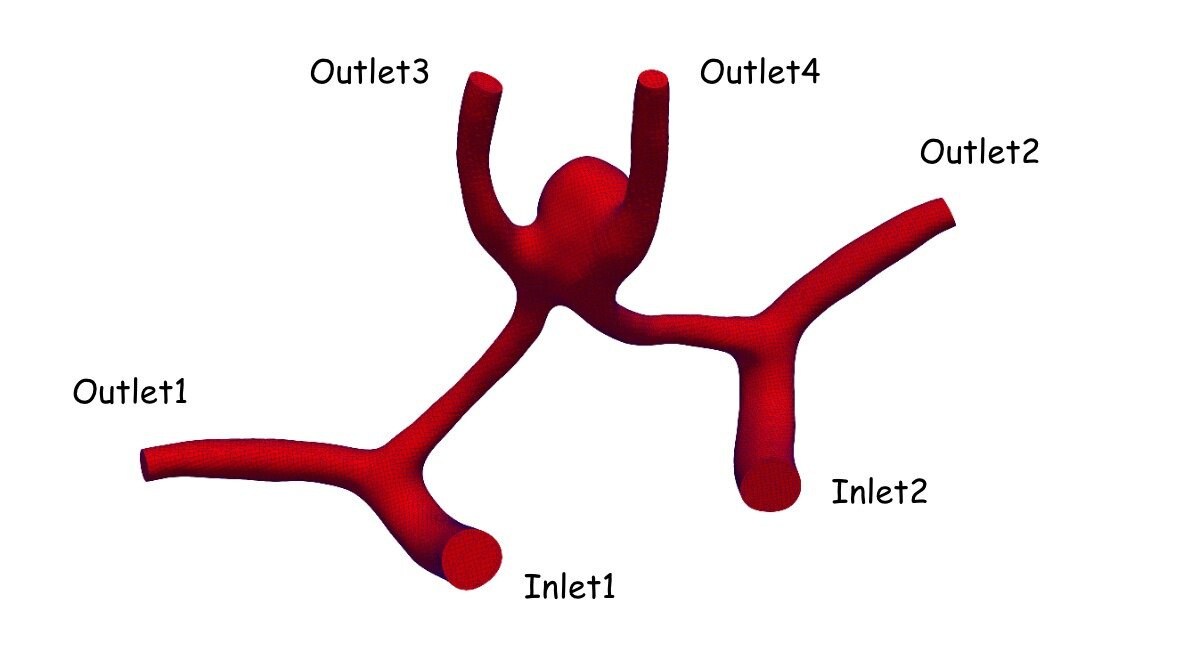
Figure 1: Patient-specific vascular geometry and inlet/outlet boundaries.
Blood is represented as an incompressible Newtonian fluid with a density of \(1050\,\mathrm{kg\,m^{-3}}\) and a dynamic viscosity of \(3.5\times10^{-3}\,\mathrm{Pa\,s}\). A representative pulsatile internal carotid artery flow-rate waveform based on values reported in the literature is prescribed at both inlets (Figure 2). Each of the four outlets uses a three-element Windkessel condition (windkesselPressure in 0/fluid/p) to represent the downstream vasculature. The waveform is not patient-specific; consequently, the case demonstrates the numerical workflow and is not intended as a clinically validated prediction.
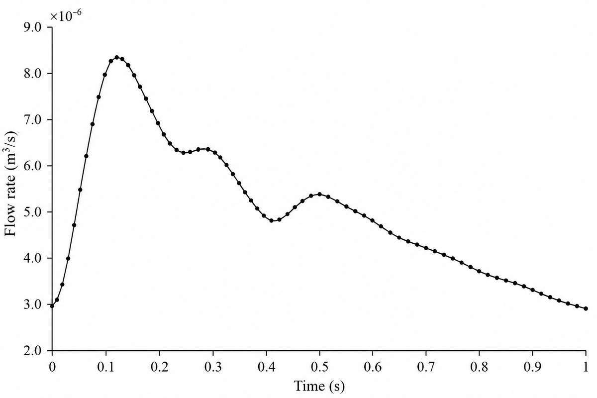
Figure 2: Prescribed inlet volumetric flow-rate waveform over one cardiac cycle.
The arterial wall is represented as a linear-elastic material with a density of \(1200\,\mathrm{kg\,m^{-3}}\), Young's modulus of \(640\,\mathrm{kPa}\) and Poisson's ratio of \(0.45\). A uniform wall thickness of \(0.3\,\mathrm{mm}\) is discretised using three cells through the thickness.
Mesh Generation
The vascular surface is converted from STL to the .fms format using
surfaceFeatureEdges geometry.stl geometry.fms
and stored in constant/triSurface. The fluid mesh is generated by cartesianMesh using system/meshDict. The solid arterial-wall mesh is then created by extruding the fluid wall patch using extrudeMesh and system/extrudeMeshDict.
Minimal root-level fvSchemes and fvSolution dictionaries are included because the standard extrudeMesh utility requires them when constructing its temporary default-region mesh. The simulation itself uses the region-specific dictionaries under system/fluid and system/solid. After extrusion, the exposed inner face of the extruded mesh is named innerWall (via exposedPatchName in system/extrudeMeshDict), and createPatch with system/createPatchDict.solid renames the outer face to outerWall.
Numerical Approach
- Fluid: incompressible Newtonian flow using
pimpleFluid. - Solid: total-displacement linear-geometry formulation with a linear-elastic material, solved with PETSc SNES using a Jacobian-free Newton-Krylov (JFNK) approach [3]. HYPRE BoomerAMG preconditions the linear solves.
- Coupling: partitioned fluid-solid interaction using fixed relaxation and a Robin pressure boundary condition. This added-mass procedure improves the stability of the partitioned coupling for the strongly coupled blood-wall system [2]. The Robin coefficient
rho_s*hsis set by thesecanthsModel(the default), which seeds the solid virtual thickness from the local wall thickness and then rescales it using the solid and fluid interface impedances measured between FSI iterations. It generally finds a good coefficient on its own, so no case-specific value has to be tuned, which is why it is used here. A hand-tuned constant also works well when a good value is known for the geometry: this case previously usedconstantHs 5e-4, which converges at a comparable rate: over the first 2000 time steps, i.e. through the initial transient and systole, it needs 2.62 FSI correctors per time step against 2.48 forsecant. The case permits up to 30 FSI correctors per time step. ThefixedRelaxationcoupling uses a relaxation factor of 1.0, i.e. no additional under-relaxation is applied, as the Robin condition already provides the required stability; the Robin-Neumann coupling is designed for such unrelaxed iterations, and Aitken or IQN-ILS acceleration is not recommended with it. - Interface:
wallin the fluid region andinnerWallin the solid region. - Duration: one cardiac cycle of \(1\,\mathrm{s}\).
The fixed time step is \(5\times10^{-5}\,\mathrm{s}\), giving 20,000 time steps over the cardiac cycle. As the time step is fixed, the Courant number follows the flow-rate waveform: over the cycle it peaks at 8.84 near peak systole (\(t\approx0.098\,\mathrm{s}\)), with a cycle-averaged value of 4.32. The implicit PIMPLE fluid solution and the FSI coupling remain stable at these Courant numbers, requiring an average of 1.8 FSI correctors per time step (see Figure 6).
The endTime in system/controlDict is currently 1, which corresponds to one cardiac cycle. To simulate additional cycles, increase endTime; for example, endTime 4; runs four cycles. The inlet-flow-rate table in 0/fluid/U uses outOfBounds repeat;, so the waveform repeats for each additional cycle.
Using a Nonlinear Geometry (Finite Strain) Formulation
The case is configured with a linear geometry (small strain, small rotation) solid formulation. Switching to a nonlinear geometry (finite strain) formulation requires only two changes:
-
In
constant/solid/solidProperties, change the solid model fromlinearGeometryTotalDisplacementto a nonlinear geometry model, for examplenonLinearGeometryTotalLagrangianTotalDisplacement, and rename the corresponding...Coeffssub-dictionary to match:solidModel nonLinearGeometryTotalLagrangianTotalDisplacement; nonLinearGeometryTotalLagrangianTotalDisplacementCoeffs { solutionAlgorithm PETScSNES; predictor yes; stabilisation { momentum { type RhieChow; scaleFactor 0.5; } } } -
In
constant/solid/mechanicalProperties, replace the small-strain mechanical law with a finite-strain law, for exampleneoHookeanElastic:mechanical ( artery { type neoHookeanElastic; rho rho [1 -3 0 0 0 0 0] 1200; E E [1 -1 -2 0 0 0 0] 640e3; nu nu [0 0 0 0 0 0 0] 0.45; } );The
neoHookeanElasticlaw takes the sameEandnuparameters aslinearElastic, so it needs no additional material data. Other finite-strain laws, such asStVenantKirchhoffElastic, may be used in the same way. Note that the mechanical law must be consistent with the solid model: small-strain laws are for linear geometry solid models, whereas finite-strain laws are for nonlinear geometry solid models.
No changes are needed to the fluid settings, the FSI coupling settings, or the boundary conditions. For the wall stiffness and pressure levels used here, the wall strains remain small, and the nonlinear geometry solution is close to the linear geometry one; the finite-strain formulation becomes important for larger deformations, such as softer walls or higher transmural pressures.
Expected Results
The flow divides between the arterial branches and develops a recirculating, lower-velocity region inside the aneurysm sac. The pressure and wall shear stress vary spatially across the vascular surface, while the structural solution predicts elevated wall stress around the aneurysm region. The images below show representative fields from the simulation.
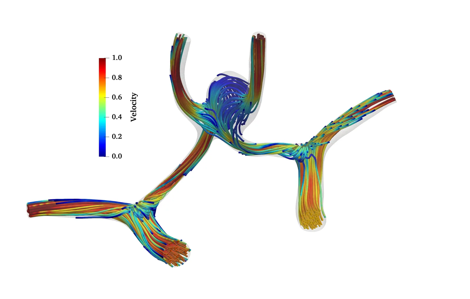
Figure 3: Fluid velocity streamlines coloured by velocity magnitude.
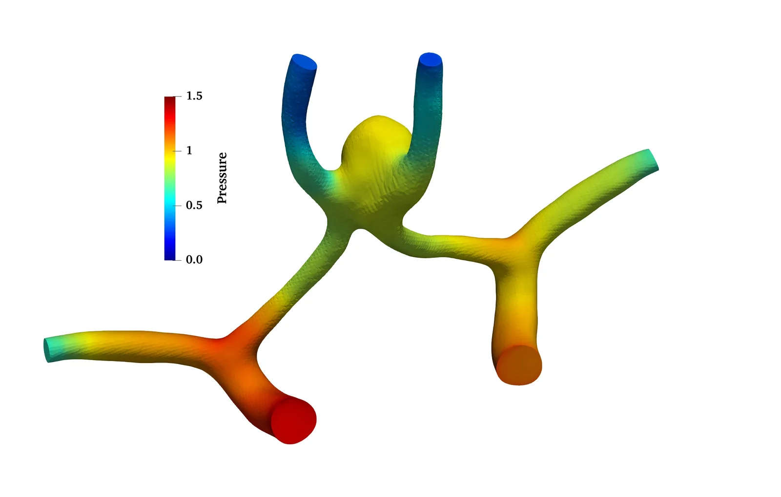
Figure 4: Pressure distribution in the fluid domain.
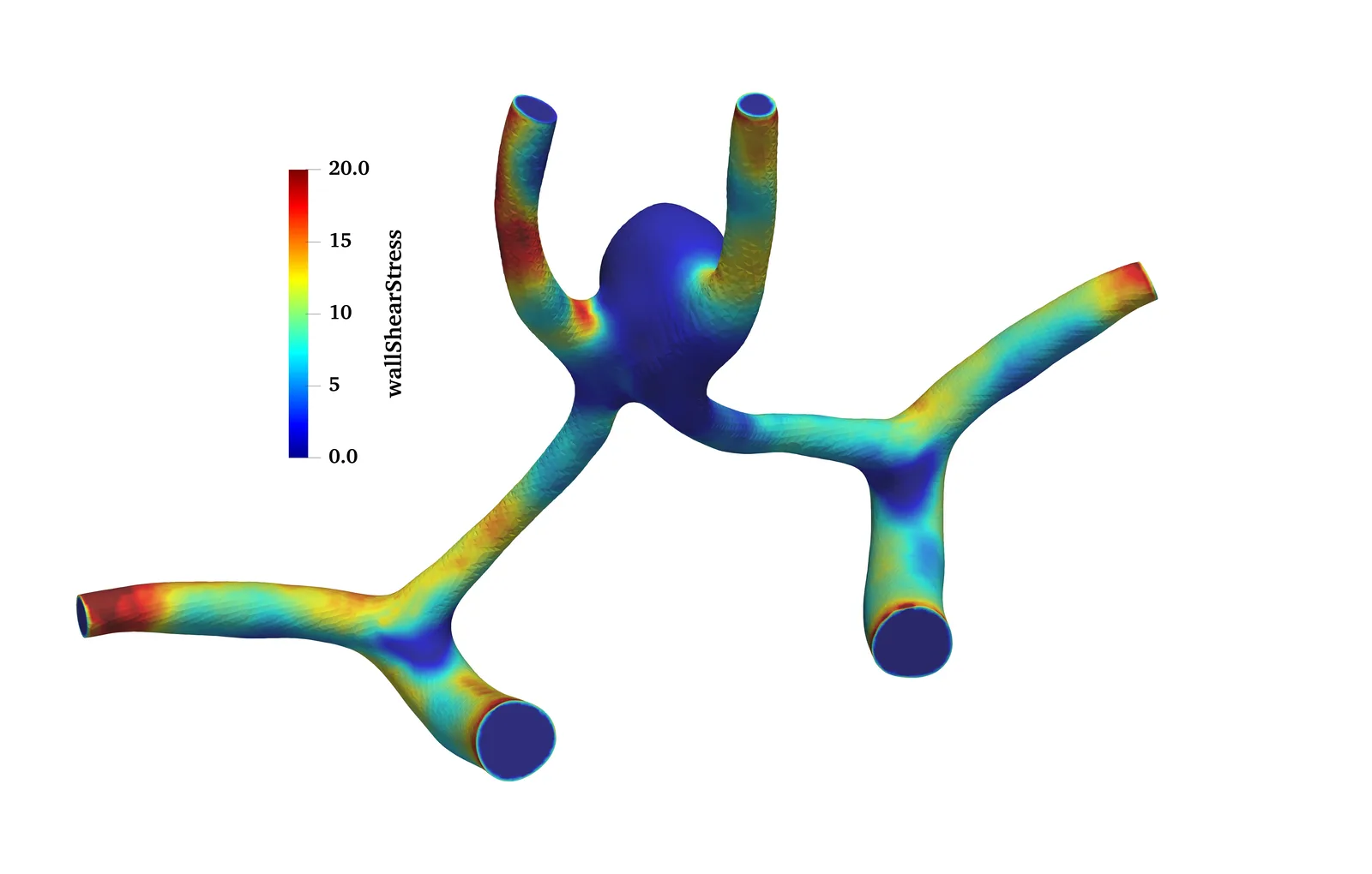
Figure 5: Wall shear stress distribution on the vascular wall.
Video 1: Time evolution of the equivalent (von Mises) stress distribution in the arterial wall over a cardiac cycle. The deformation has been scaled by a factor of 5.
The number of FSI (outer) iterations performed in each time step is recorded in postProcessing/fsiResiduals.dat. Allrun post-processes this file with fsiIterations.gnuplot to produce fsiIterations.pdf and fsiIterations.png (this step is skipped if gnuplot is not installed).
The surfaceFieldValue function objects in system/controlDict also record the signed mass flow through the two inlets, the four outlets, and the fluid FSI patch. interfaceAbsoluteMassFlowRate records the sum of the magnitudes of the face fluxes on the FSI patch, so local leakage cannot be hidden by cancellation in the signed interface flow. The values are calculated from the mesh-relative volumetric flux phi and scaled by the blood density of \(1050\,\mathrm{kg\,m^{-3}}\) to give mass flow in \(\mathrm{kg\,s^{-1}}\).
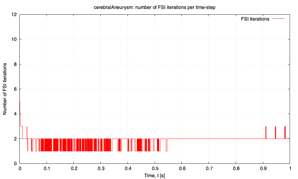
Figure 6: Number of fluid-solid interaction iterations per time step over one cardiac cycle.
The partitioned coupling is inexpensive once the initial transient has passed: 11 iterations are needed in the first time step, after which the count settles to one or two iterations, averaging 1.3 over the cardiac cycle. In the measured run below, 77% of the time steps converged in a single FSI corrector and a further 19% in two. The limit of 30 FSI correctors per time step is never reached.
Running the Case
From the tutorial directory, run
./Allclean
./Allrun parallel
The case is configured for 16 subdomains by default (system/decomposeParDict and its fluid and solid counterparts); change numberOfSubdomains in all three to run on a different number of cores. Omit parallel to run in serial.
As a representative run time, the full cardiac cycle (20,000 time steps of \(5\times10^{-5}\,\mathrm{s}\)) completed in 5633 s of solver time (approximately 1 hour 34 minutes) using 8 cores, i.e. with numberOfSubdomains reduced from the default 16 to 8. The hardware was an Apple Mac Studio with an M1 Ultra chip (20 cores: 16 performance and 4 efficiency) and 64 GB of unified memory, running macOS 26.5 and OpenFOAM v2412. This timing excludes mesh generation, which takes a few seconds, and the reconstruction of the parallel results.
Performance varies with hardware and through the cardiac cycle, as the cost per time step follows the FSI iteration count shown in Figure 6.
The Allrun workflow is
cartesianMesh -> extrudeMesh -> createPatch -> checkMesh -> solids4Foam
Regression Test
The case includes a regressionTest.sh script:
./regressionTest.sh
Because the full cardiac cycle takes hours, the script copies the case inputs to cerebralAneurysm/regressionTests/main/, reduces endTime to \(5\times10^{-4}\,\mathrm{s}\) (the first 10 time steps of the initial transient) and runs the case in serial there; the tutorial directory itself is untouched. On the hardware above, the check takes approximately two minutes.
The following quantities are then compared with stored reference values, within loose tolerances:
- the largest
innerWalldisplacement component frompostProcessing/0/solidDisplacementsinnerWall.dat, - the
innerWallnormal force frompostProcessing/0/solidForcesinnerWall.dat.
Pass --check-only to re-check an existing regression run without re-running the case. If PETSc or cartesianMesh is unavailable, Allrun exits silently and the script skips the checks rather than reporting a failure.
References
- N. M. Wilson, A. K. Ortiz, and A. B. Johnson, "The Vascular Model Repository: A Public Resource of Medical Imaging Data and Blood Flow Simulation Results," Journal of Medical Devices, 7(4), 040923 (2013). https://doi.org/10.1115/1.4025983. Model
0199_H_CERE_CA, Vascular Model Repository. - Ž. Tuković, M. Bukač, P. Cardiff, H. Jasak, and A. Ivanković (2019). "Added Mass Partitioned Fluid–Structure Interaction Solver Based on a Robin Boundary Condition for Pressure." In: J. Nóbrega and H. Jasak (eds), OpenFOAM®. Springer, Cham. https://doi.org/10.1007/978-3-319-60846-4_1.
- P. Cardiff, D. Armfield, Ž. Tuković, and I. Batistić, "A Jacobian-Free Newton-Krylov Method for Cell-Centred Finite Volume Solid Mechanics," International Journal for Numerical Methods in Engineering, 127(3), e70268 (2026). https://doi.org/10.1002/nme.70268.