Spherical cavity under uniaxial tensions: sphericalCavity

Prepared by Philip Cardiff and Ivan Batistić

Tutorial Aims

• Demonstrate how to perform a 3D linear-static stress analysis in solids4foam
• Demonstrate the process of meshing using the Gmsh meshing utility and OpenFOAM polyDualMesh utility
• Demonstrates using the solids4foam solid solver based on the PETSc SNES nonlinear solver

Case Overview

This classic 3-D problem consists of a spherical cavity with radius $a = 0.2$ m (Figure 1) in an infinite, isotropic linear elastic solid ($E = 200$ GPa, $\nu = 0.3$). Far from the cavity, the solid is subjected to a tensile stress $\sigma_{zz} = T = 1$ MPa, with all other stress components zero. The analytical expressions for stress are derived by Southwell and Gough [1], while expressions for displacement are derived by Goodier [2]. The problem is characterised by a localised stress concentration near the cavity on the plane perpendicular to the loading, which drops off rapidly away from the cavity. The computational solution domain is taken as one-eighth of a $1 \times 1 \times 1$ m cube aligned with the Cartesian axes, with one corner at the sphere's centre. The problem is axisymmetric but is analysed here using a 3-D domain. The analytical tractions are applied at the far boundaries of the domain to mitigate the effects of finite geometry. They are defined with analyticalSphericalCavityTraction boundary conditions, which require geometry (cavity radius), loading (far-field traction), and material properties (Poisson's ratio):

    patch
    {
        type            analyticalSphericalCavityTraction;
        farFieldTractionZ 1e6;
        cavityRadius    0.2;
        nu              0.3;
        value           uniform (0 0 0);
    }

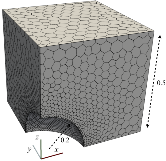
Figure 1: Spherical cavity case geometry and mesh (4 555 cells).

Expected Results

The analytical expressions for the stress distributions around the cavity, first derived by Southwell and Gough [1], are:

where $a$ is the hole radius, $T$ is the distant stress applied in the $z$ direction, $\nu$ is the Poisson's ratio, $r^2 = x^2 + y^2$ is the cylinderical radial coordinate, $R^2 = r^2 + z^2$ is the spherical radial coodinate, and $x$, $y$, $z$ are the Cartesian coordinates.

The displacement distributions were later derived by Goodier [2]: $$ u_r = -\frac{A}{r^2} - \frac{3B}{r^4}

• \left[ \frac{5-4\nu}{1-2\nu} \frac{C}{r^2}-9\frac{B}{r^4} \right]\cos (2\theta), $$

where the constants $A$, $B$ and $C$ are defined as follows: \(\frac{A}{a^3} = -\frac{T}{8\mu}\frac{13-10\nu}{7-5\nu}, \qquad \frac{B}{a^5} = -\frac{T}{8\mu}\frac{1}{7-5\nu}, \qquad \frac{C}{a^3} = -\frac{T}{8\mu}\frac{5(1-2\nu)}{7-5\nu}.\) and $\mu$ is the shear modulus.

The analytical solution is generated alongside solution fields using the function object sphericalCavityAnalyticalSolution located in the system/controlDict, where one needs to input geometry, laoding and material data:

functions
{
    cavityAnalytical
    {
        type sphericalCavityAnalyticalSolution;
        farFieldTractionZ 1e6;
        cavityRadius 0.2;
        E 200e9;
        nu 0.3;
        cellDisplacement yes;
        pointDisplacement no;
        cellStress yes;
        pointStress no;
    }
}

The distribution of $zz$-component of stress field (sigma[ZZ]) is shown in Figure 2.

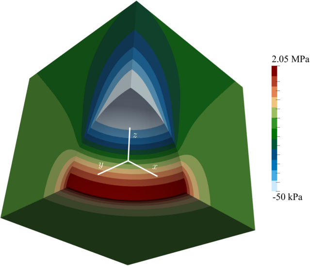
Figure 2: $\sigma_{zz}$ stress distribution.

Running the Case

The tutorial case is located at solids4foam/tutorials/solids/linearElasticity/sphericalCavity. The case can be run using the included Allrun script, i.e. ./Allrun. In this case, the Allrun creates the unstructured tetrahedral mesh using the Gmsh meshing utility, followed by conversion to its dual polyhedral representations using the OpenFOAM polyDualMesh utility:

   # Create mesh with gmsh
    solids4Foam::runApplication gmsh -3 -format msh2 sphericalCavity.geo
    solids4Foam::runApplication gmshToFoam sphericalCavity.msh
    solids4Foam::runApplication polyDualMesh 30 -overwrite
    solids4Foam::runApplication combinePatchFaces 45 -overwrite
    solids4Foam::runApplication changeDictionary

The case is setup to use the small strain (linear geometry) cell-centred finite volume solid solver based on the PETSc SNES nonlinear solver, as defined in constant/solidProperties:

solidModel     linearGeometryTotalDisplacement;

linearGeometryTotalDisplacementCoeffs
{
    // Solution algorithm
    //solutionAlgorithm implicitSegregated;
    solutionAlgorithm PETScSNES;
    //solutionAlgorithm explicit;

    // PETSc options file used by PETScSNES
    optionsFile petscOptions.snes;
}

Here, the linearGeometryTotalDisplacement solid solver can adopt one of three solution algorithms:

• implicitSegregated: the standard segregated solution procedure, where each displacement component equation is solved separately.
• PETScSNES: using the PETSc SNES nonlinear solver, which is provided with the a compact stencil, approcimate Jacobian. Various solution procedures can be specified through the optionsFile petscOptions.snes; file included in the case. The Jacobian-free Newton-Krylov approach is typically faster than the segregated approach, as examined in Cardiff et al. (2025) [3].
• explicit: fully-explicit (matrix-free) approach, where the time step size is limited by the stand CFL criterion.

References

[1] Southwell, R.V., Gough, H.J.: Vi. On the concentration of stress in the neighbourhood of a small spherical flaw; and on the propagation of fatigue fractures in "statistically isotropic" materials. The London, Edinburgh, and Dublin Philosophical Magazine and Journal of Science 1(1), 71–97 (1926)

[2] Goodier, J.N.: Concentration of stress around spherical and cylindrical inclusions and flaws. Journal of Applied Mechanics 1(2), 39–44 (1933)

[3] Cardiff, P., Armfield, D., Tukovic, Z., Batistic, I.: Assessing the potential of Jacobian-free Newton-Krylov methods for cell-centred finite volume solid mechanics. Preprint, arXiv