Filling an elastic container with a viscous fluid: `fillingElasticContainer`

Prepared by Philip Cardiff, Amirhossein Taran, Ivan Batistić

Tutorial Aims

This tutorial case demonstrates two-phase fluid–structure interaction involving the filling of a highly deformable elastic container with a viscous fluid, where added-mass effects are prominent.

Case Overview

The case is inspired by, and closely related to, the benchmark problems presented in the literature on Lagrangian and partitioned fluid-solid interaction methods [1-3]. In contrast to the original benchmark configurations, this implementation explicitly includes two fluid phases (water and air). As a result, the behaviour is not strictly identical to the single-phase reference cases [1-3]; in particular, trapped air pockets may influence the subsequent fluid motion and solid deformation.

A volume of viscous fluid falls under gravity from a rigid reservoir into a thin, highly deformable, low-density elastic container (Figure 1). The impact and subsequent filling induce large deformations of the elastic structure, followed by chaotic oscillatory motion, before the system comes to a rest.

Key features of the problem:

Strong two-way fluid–structure interaction
Large solid deformations and displacements
Free-surface flow
Two-phase flow (water + air)
Significant added-mass effects: fluid-to-solid density ratio of 50.

The problem geometry and material parameters are based on the benchmark studies from the literature [1-3], with adaptations required for the two-phase formulation used here. In particular, a second fluid (air) phase is assumed, and, consequently, atmospheric vents are added instead of walls at the top of the elastic container to allow the air to escape as the viscous fluid drops from the funnel.

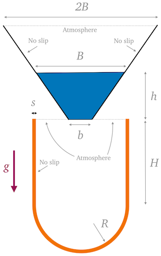
Figure 1: Fluid and solid computational domains and boundary conditions

Figure 1: Fluid and solid Computational domains and boundary conditions.

The default tutorial case contains a relatively coarse mesh with \(4\,000\) fluid cells and \(480\) solid cells.

The adopted material parameters are given below:

Table 1: Problem Physical Parameters

Category	Parameter	Value	Units
Geometry	Rigid container top side	4.87	m
	Rigid container bottom side, \(b\)	1.30	m
	Rigid container height, \(h\)	2.50	m
	Elastic container straight side, \(H\)	3.75	m
	Elastic container cap radius, \(R\)	2.25	m
	Elastic container thickness, \(s\)	0.20	m
	Gravity, \(g\)	9.81	m/s\(^2\)
Solid	Density, \(\rho_s\)	20	kg/m\(^3\)
	Young's modulus, \(E_s\)	\(2.1\times10^7\)	Pa
	Poisson's ratio, \(\nu_s\)	0.3
Fluid	Phase 1 density, \(\rho_{f_1}\)	1000	kg/m\(^3\)
	Phase 1 dynamic viscosity, \(\mu_{f_1}\)	100	Pa·s
	Phase 2 density, \(\rho_{f_2}\)	1	kg/m\(^3\)
	Phase 2 dynamic viscosity, \(\mu_{f_2}\)	\(1.48\times10^{-5}\)	Pa·s
	Surface tension coefficient, \(\sigma\)	0	N/m

Numerical approach

Fluid: two-phase incompressible flow (water + air) using an arbitrary Lagrangian-Eulerian volume of fluid formulation (interFoam)
Solid: nonlinear hyperelastic total Lagrangian solid formulation with Jacobian-free Newton-Krylov solution algorithm [5]
Coupling: partitioned FSI framework with Robin-Neumann coupling [4]
Time integration: transient

Compared to the original single-phase benchmarks, the inclusion of air introduces additional physical effects, such as air entrapment dynamics, which can alter the transient response.

This case therefore serves both as:

A reproduction (with modifications) of a well-established fluid-solid interaction benchmark, and
A demonstration of two-phase fluid-solid interaction capabilities within solids4foam, where added-mass effects are prominent, i.e. when the fluid density is similar to or less than the solid density.

Running the case

From the case directory:

./Allrun

To clean the case:

./Allclean

Results

Typical fields of interest include:

alpha.water (phase distribution)
Displacement and deformation of the elastic container
Fluid pressure and velocity fields

Video 1 shows the Time evolution of the phase distribution field in the fluid and the displacement magnitude field in the solid

Video 1: Time evolution of the phase distribution field in the fluid and the displacement magnitude field in the solid.

A commonly reported metric for this benchmark is the vertical displacement of the container apex as a function of time. This data is recored in the case via the solidPointDisplacement function object, placed in system/controlDict.

functions
{
    disp
    {
        type    solidPointDisplacement;
        point   (0 -6.0 0);
    }
}
  

The solidPointDisplacement function object records the displacement history of the selected container apex point and write them to the file:

postProcessing/0/solidPointDisplacement_disp.dat

The displacement vs time are shown in Figure 2, where the results from two solids4foam mesh densities are shown; close agreement are seen with the single-phase results from the literature for the initial displacement spike.

Figure 2: Displacement of the container apex point vs time. Adapted from [3].

Figure 2: Displacement of the container apex point vs time.

Figure 3 shows the number of fluid-solid interaction coupling iteration per time step (mesh with \(2\,000\) fluid and \(400\) solid cells), showing that the adopted partitioned Robin-Neumann coupling approach requires between 3 and 6 iterations in all time steps apart from 11 in the first time step: this highlights the robustness and efficiency of the Robin-Neumann coupling approach in this high added-mass scenario.

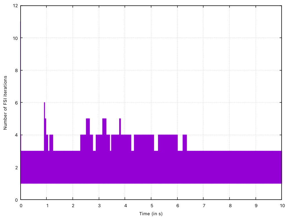
Figure 3: Number of fluid-solid interaction coupling iterations vs time.

Figure 3: Number of fluid-solid interaction coupling iterations vs time.

The original benchmark problems reported in the literature typically consider a single-phase viscous fluid, neglecting the presence of air.

In this solids4foam case:

Air is explicitly modelled as a second phase.
A full air pocket may become trapped during filling.
This can lead to differences in:
- transient pressure fields,
- oscillation frequencies,
- damping behaviour,
- final equilibrium configuration.

As a result, while qualitative agreement with published results is expected, exact quantitative agreement should not be assumed.