Slender Cantilever in Bending: cantilever2d
Prepared by Philip Cardiff
Tutorial Aims
- Verify the accuracy of solids4foam solid models for a slender cantilever in bending.
- Compare the performance of cell-centred and vertex-centred discretisatins and segregated and coupled solution algorithms for bending dominated scenarios.
- Demonstrate how to set up a high-order cell-centred discretisation.
- Demonstrates the slow convergence of the solution algorithm for high aspect ratio geometry undergoing bending.
Case Overview
The test case geometry consists of a rectangular beam \(L \times D\) m, where \(L = 2\) m and \(D = 0.1\) m, with a Young's modulus \(E\) of 200 GPa and a Poisson's ratio (\(\nu\)) of 0.3. A uniform quadrilateral mesh with \(5\,120\) cells is employed. The beam is fixed on the left boundary and a load of \(100\) kN is applied to the right. There are no body forces. The problem is solved as static, using one loading increment. From Timoshenko beam theory [1], the analytical solution for the \(x\) and \(y\) components of the displacement field are given as:
\[u_x = -\frac{P y}{6 E I} \left[ (6L - 3x)x + (2 + \nu)\left(y^2 - \frac{D^2}{4}\right) \right], \\ u_y = -\frac{P}{6 E I} \left[ 3\nu y^2 (L - x) + (4 + 5\nu)\frac{D^2 x}{4} + (3L - x)x^2 \right]\]where \(I = \frac{D^3}{12}\) m\(^4\) is the second moment of area of the cross-section, and the origin is assumed at the centre of the fixed (left) boundary. The analytical stresses are
\[\sigma_{xx} = \frac{P (L - x) y}{I}, \\ \sigma_{yy} = 0, \\ \tau_{xy} = -\frac{P}{2I} \left[ \frac{D^2}{4} - y^2 \right].\]For consistency with the analytical problem (see [1]), the analytical stress is applied to the right end of the bar, while the analytical displacement is applied to the left end.
A custom cantileverAnalyticalSolution function object is added to the controlDict to calculate the analytical solutions for displacement and stress and compute the errors:
functions
{
    cantileverAnalytical
    {
        type cantileverAnalyticalSolution;
        P 0.1e6;
        E 200e9;
        nu 0.3;
        L 2;
        D 0.1;
        cellDisplacement yes;
        pointDisplacement yes;
        cellStress yes;
        pointStress no;
    }
}
In solids4foam, there are several solid models which can solve this problem; here, five approaches are considered:
- A cell-centred finite volume approach with a Jacobian-free Newton-Krylov solution algorithm [2]. This is the default approach in the case, and is selected by specifying
solidModel linearGeometryTotalDisplacement;inconstant/solidProperties, withsolutionAlgorithm PETScSNES;inlinearGeometryTotalDisplacementCoeffs. - A cell-centred finite volume approach with a segregated solution algorithm. This approach employs the same discretisation as in approach 1, but solves the governing equations using the more common (in OpenFOAM) segregated algorithm. This approach is selected by specifying
solidModel linearGeometryTotalDisplacement;inconstant/solidProperties, withsolutionAlgorithm implicitSegregated;inlinearGeometryTotalDisplacementCoeffs. - A vertex-centred finite volume approach with an exact Jacobian coupled solution algorithm [3]. This approach is selected by specifying
solidModel vertexCentredLinearGeometry;inconstant/solidProperties, withsolutionAlgorithm PETScSNES;andapproximateJacobian no;invertexCentredLinearGeometryCoeffs. - A cell-centred finite volume approach with an exact Jacobian coupled solution algorithm [4]. This approach is selected by specifying
solidModel coupledUnsLinearGeometryLinearElastic;inconstant/solidProperties. - A cell-centred high-order finite volume approach with a Jacobian-free Newton-Krylov solution algorithm. This approach uses the
linearGeometryTotalDisplacementsolid model withsolutionAlgorithm PETScSNES;and a high-order residual calculation [5]. It is selected by specifyingsolidModel linearGeometryTotalDisplacement;inconstant/solidProperties, withhighOrderResidual true;in thehighOrderCoeffssub-dictionary. WhenhighOrderJacobian false;is used, the solver uses the same second-order Laplacian as approach 1 as a physical preconditioner. Alternatively,highOrderJacobian true;can be used to assemble the high-order Jacobian; this affects the timing but not the accuracy.
Approach 4 uses simplified uniform displacement (left) and uniform traction (right) boundary conditions, which give similar results for coarse/medium meshes but converge to a slightly different result than the analytical solution.
Running the Case
The tutorial case is located at solids4foam/tutorials/solids/linearElasticity/cantilever2d. The case can be run using the included Allrun script, i.e. > ./Allrun. In this case, the Allrun script optionally takes an argument which specifies which specifies the solution approach:
./Allrun                # Defaults to approach 1 (petscSnes)
./Allrun petscSnes      # Approach 1
./Allrun segregated     # Approach 2
./Allrun vertexCentred  # Approach 3
./Allrun unsCoupled     # Approach 4
./Allrun highOrder      # Approach 5
The Allrun script starts by updating the files in the case to match the selected approach; the following files are updated: 0/D, 0/pointD, constant/solidProperties, system/fvSchemes, and system/fvSolution. Subsequently, the mesh is created with blockMesh, following by running the solver solids4Foam.
Results
The von Mises stress (sigmaEq) distribution for the mesh with \(320 \times 16\) cells is shown in Figure 1, generated with the default case settings.
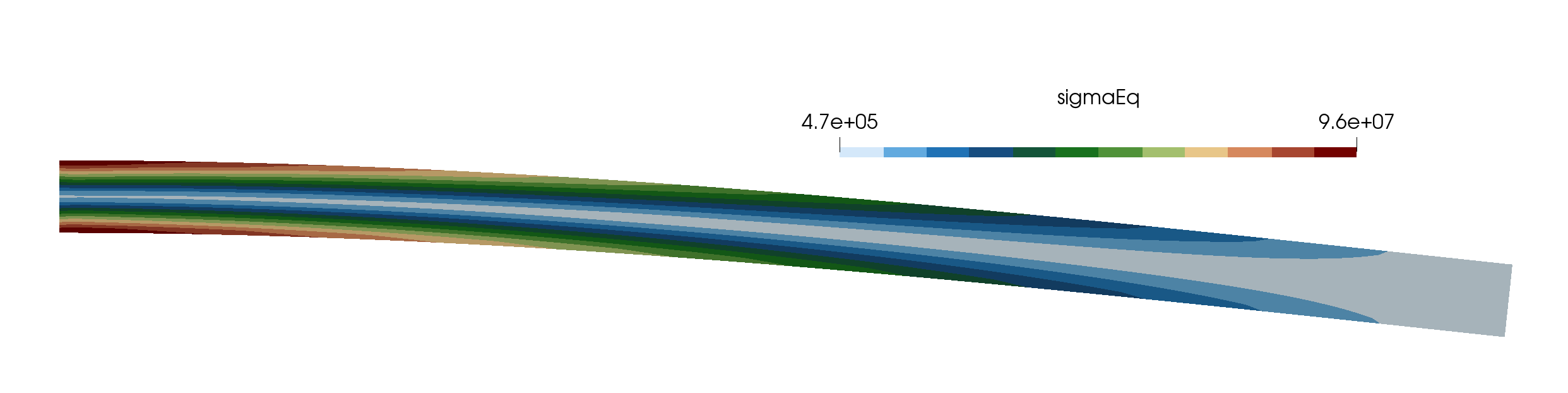
Figure 1: Von Mises stress distribution (deformation scale factor = 10).
Table 1 lists the wall-clock times rounded to the nearest second for the different approaches, where the segregated approach is significantly slower than the coupled approaches for this problem (\(123\) s vs \(1\) s). Such significant differences in efficiency are typical other static problems where high aspect ratio geometry is undergoing bending. However, for transient cases or where the aspect ratio is lower or bending effects are small, then the segregated approach can provide similar (or better) efficiency than the coupled approaches.
Table 1: Wall-clock time (in s)
| Approach | Mesh (# cells) | Time (in s) |
|---|---|---|
| 1 | 5120 | 1 |
| 2 | 5120 | 123 |
| 3 | 5120 | 1 |
| 4 | 5120 | - |
| 5 | 5120 | 1 |