Hole in a Infinite Plate Subjected to Remote Stress: plateHole
Prepared by Philip Cardiff and Ivan Batistić
Tutorial Aims
- Demonstrate the solver accuracy for a linear elastic test case.
Case Overview
In this case, a thin, infinitely large plate with a circular hole is subjected to uniaxial tension of \(\sigma_{xx} = T = 1\) MPa, see Figure 1. Owing to the symmetry of the geometry and loading, only one quarter of the plate is modelled. To minimise the influence of the finite computational boundaries, the exact tractions obtained from the analytical solution [1,2,3] are prescribed on the outer edges BC and CD. They are defined with analyticalPlateHoleTraction boundary conditions, which require geometry (hole radius) and loading (far-field traction):
right
{
    type            analyticalPlateHoleTraction;
    farFieldTractionX 1e6;
    holeRadius      0.5;
    value           uniform (0 0 0);
}
Symmetry boundary conditions are applied on boundaries AB and DE, while zero traction is specified on the hole boundary. The material properties are defined by a Young's modulus of \(E = 200 GPa\) and a Poisson's ratio of \(\nu = 0.3\). Gravitational and inertial effects are neglected, and the case is solved using one loading increment.
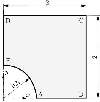
Figure 1 - Problem geometry [3]
Expected Results
The analytical solution for the stress field is [1,2,3]:
\[\sigma_{xx} = T \left[ 1 - \dfrac{R^2}{r^2} \left( \dfrac{3}{2}\cos(2\theta) +\cos (4\theta)\right) + \dfrac{3}{2}\dfrac{R^4}{r^4}\cos (4\theta) \right],\] \[\sigma_{yy} = T \left[ - \dfrac{R^2}{r^2} \left( \dfrac{1}{2}\cos(2\theta) -\cos (4\theta)\right) - \dfrac{3}{2}\dfrac{R^4}{r^4}\cos (4\theta) \right],\] \[\sigma_{xy} = T \left[ - \dfrac{R^2}{r^2} \left( \dfrac{1}{2}\sin(2\theta) +\sin (4\theta)\right) + \dfrac{3}{2}\dfrac{R^4}{r^4}\sin (4\theta) \right].\]where \(r=\sqrt{x^2+y^2}\) and \(\theta=\tan^{-1}(y/x)\) are the usual polar co-ordinates. \(R\) is the hole radius. Stresses in cylindrical coordinates: $$ \sigma_r = \frac{T}{2}\left( 1-\frac{a^2}{r^2}\right)
- \frac{T}{2} \left( 1+\frac{3a^4}{r^4} - \frac{4a^2}{r^2} \right)cos(2\theta), $$
Displacement field in cartesian coordinates: \(u_x = \frac{Ta}{8\mu}\left( \frac{r}{a}(\kappa+1)\cos\theta+\frac{2a}{r} \left((1+\kappa)\cos(\theta)+\cos (3\theta)\right) -\frac{2a^3}{r^3}\cos(3\theta) \right),\)
\[u_y = \frac{Ta}{8\mu}\left( \frac{r}{a}(\kappa-3)\sin\theta+\frac{2a}{r} \left((1-\kappa)\sin(\theta)+\sin (3\theta)\right) -\frac{2a^3}{r^3}\sin(3\theta) \right),\]where \(a\) is hole radius, \(T\) is far field traction in \(x\) direction, \(\nu\) is Poisson's ratio, \(\mu\) is shear modulus and \(\kappa\) parameter is equal to \(3-4\nu\).
A custom plateHoleAnalyticalSolution function object is added to the controlDict to calculate the analytical solutions for displacement and stress and compute the errors:
plateHoleAnalyticalSolution1
{
    type          plateHoleAnalyticalSolution;
    farFieldTractionX 1e6;    // Farfield sigma_xx
    holeRadius    0.5;        // Hole radius
    E             200e+9;     // Young modulus
    nu            0.3;        // Poissons ratio

    //Optional
    cellDisplacement true;
    pointDisplacement true;
    cellStress true;
    pointStress true;
}
The function object prints the average \(L_1\), \(L_2\), and \(L_\infty\) norms for the stress components (\(\sigma_{xx}\), \(\sigma_{yy}\), and \(\sigma_{xy}\)) and for the displacement field:
Writing cellStressDifference field
    Component: 0
    Norms: mean L1, mean L2, LInf:
    3284.42 10421.2 105024

    Component: 1
    Norms: mean L1, mean L2, LInf:
    2100.42 6111.58 59602.5

    Component: 3
    Norms: mean L1, mean L2, LInf:
    2917.5 8547 87630.5

Writing DDifference field
    Norms: mean L1, mean L2, LInf:
    1.2549e-08 1.37329e-08 4.24642e-08
In solids4foam the error normas \(L_1\),\(L_2\) and \(L_\inf\) are defines as:
where \(\Delta \phi_i\) is the difference between expected and predicted solutions For variable \(\phi\) at computational nodes and \(N_{\text{c}}\) is the overall number of computational nodes, i.e. cells.
Running the Case
The tutorial case is located at solids4foam/tutorials/solids/linearElasticity/plateHole. The case can be run using the included Allrun script. The Allrun script optionally takes an argument which specifies the solution approach:
./Allrun             # Defaults to the segregated approach
./Allrun segregated  # Segregated second-order approach
./Allrun petscSnes   # PETSc SNES second-order approach [4]
./Allrun highOrder   # PETSc SNES high-order approach [5]
The Allrun script starts by updating the files in the case to match the selected approach; the following files are updated: constant/solidProperties, system/fvSchemes, and system/fvSolution. Subsequently, the tutorial-local library in the src directory is compiled, the mesh is created with blockMesh, followed by running the solver solids4Foam.
Any approach can be run in parallel by adding parallel as the second argument, for example:
./Allrun segregated parallel
./Allrun petscSnes parallel
./Allrun highOrder parallel
The script also supports pressure-displacement solution options (foam-extend only):
./Allrun pressureDisplacementCompressible coarse
./Allrun pressureDisplacementCompressible medium
./Allrun pressureDisplacementIncompressible coarse
./Allrun pressureDisplacementIncompressible medium
These pressure-displacement options use coupledPressureDisplacementSolid with nonLinear false in constant/solidProperties. The material law is selected as neoHookeanElastic because that law provides the pressure-displacement stress form, but with nonLinear false the case remains a linear-geometry linear-elastic plate-hole benchmark.
References
[1] [Timoshenko, Stephen. Theory of elasticity. Oxford, 1951.