Custom workflow tutorial: brakeLever

Prepared by: Ivan Batistić and Philip Cardiff

Tutorial Aims

• Provide a step-by-step process for building a custom solids4foam case from scratch. Using a brake lever as the example, the tutorial covers the complete workflow: meshing, setting up the case files, running the solver, and post-processing the results.

Prerequisites

Prerequisites for this tutorial are:

• solids4foam-v2.2
• openfoam2312
• ParaView-5.13.2

It is possible to follow the tutorial steps with other OpenFOAM and ParaView versions, but be aware of possible minor differences.

Problem description

This tutorial analyses a brake lever, as shown in the image below. The geometry has three key surfaces: a green surface where a load is applied, a yellow surface where a pin allows rotation, and a red surface where the cable end is attached. For this analysis, we will make the following assumptions:

• The red surface is fixed.
• A pressure of 50 kPa is applied to the green surface.
• The lever is made of aluminium with a Young's modulus of 70 GPa and a Poisson's ratio of 0.33.
• Gravitational effects are neglected.
• The analysis assumes small deformations and a linear elastic (Hookean) material response.

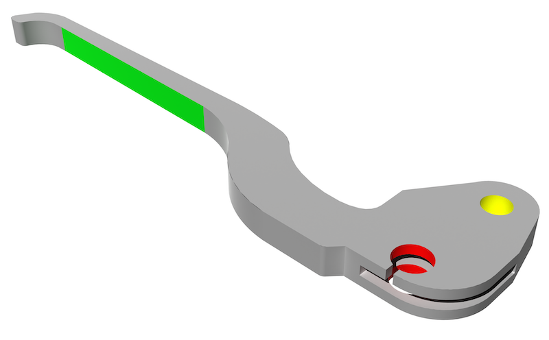
Loading (green), fixed (red) and frictionless support (yellow) surfaces

Step 1. Preparing case geometry

For convenience, we will set up the SOLIDS4FOAM_DIR variable to point to the solids4foam installation directory. Since this location is user-dependent, this will ensure that the subsequent commands are applicable to all users:

echo 'export SOLIDS4FOAM_DIR=<PATH_TO_SOLIDS4FOAM>'

where you should replace<PATH_TO_SOLIDS4FOAM> with the location of the solids4foam directory on your system. Optionally, make it permanent by adding it to ~/.bashrc:

echo 'export SOLIDS4FOAM_DIR=<PATH_TO_SOLIDS4FOAM>' >> ~/.bashrc
source ~/.bashrc

Now, create a new directory for this case and navigate into it:

mkdir brakeLever
cd brakeLever

Download and unpack the geometry:

wget https://www.solids4foam.com/tutorials/archive/lever.zip \
  && unzip lever.zip && mv lever/* . \
  && rm -rf lever lever.zip

The geometry is provided in several .stl files, each representing a different boundary patch. We will combine them into a single file for the mesher:

cat *.stl > brakeLever.stl

Before meshing, it is a good practice to inspect the geometry in ParaView. The touch command creates a dummy file that allows ParaView to recognise the folder as an OpenFOAM case.

touch case.foam && paraview case.foam

Once ParaView opens, load the brakeLever.stl file using File > Open… to view the geometry.

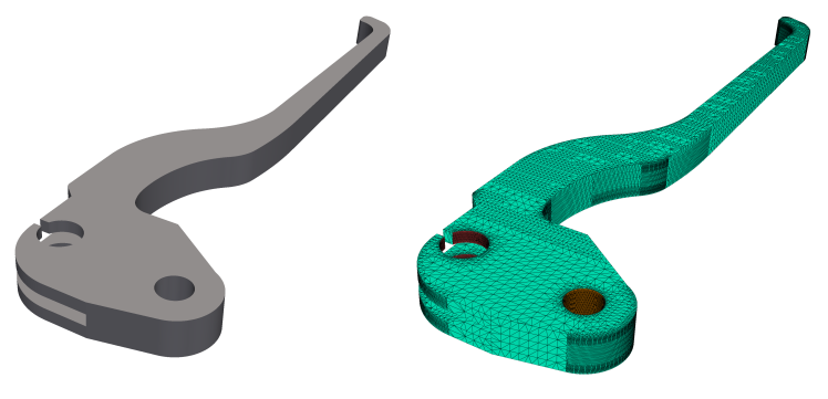
Case geometry (left) and geometry STL (right)

Step 2. Meshing using cfMesh

Before meshing, we must populate the case directory with the necessary OpenFOAM files. The most efficient way to do this is to copy the structure from a similar tutorial case. Since our simulation assumes small deformations and a linear elastic material, the cases in solids4foam/tutorials/solids/linearElasticity are a good starting point. We will use the plateHole tutorial:

cp -r $SOLIDS4FOAM_DIR/tutorials/solids/linearElasticity/plateHole/* .

The cfMesh mesher comes with OpenFOAM (OpenFOAM.com) as a sub-module, so you You need to compile it before you can use it. This can be done with the following commands:

foam
cd modules
git submodule update --init cfmesh
cd cfmesh
./Allwmake

Once the compilation is successful, return to your brakeLever case directory. Meshing with cfMesh is controlled by the system/meshDict file. We will copy a suitable example from the wobblyNewton solids4foam tutorial:

cp $SOLIDS4FOAM_DIR/tutorials/solids/linearElasticity/wobblyNewton/ \
 system/meshDict system/

Next, let us check the geometry file. The surfaceCheck utility provides statistics about the surface triangulation and its bounding box.

surfaceCheck brakeLever.stl
rm -rf *.obj

Statistics:
Triangles    : 45064 in 4 region(s)
Vertices     : 22607
Bounding Box : (-30.3771 -24.3679 -4.5) (20.3966 169.632 4.5)

Region  Size
------  ----
fixed   4716
freeRotation    7226
freeTraction    31544
load    1578


Surface has no illegal triangles.
...

The output shows that the geometry is valid, but the bounding box dimensions suggest the units are in millimetres. We need to scale the geometry to meters for our simulation. We can do this with the scaleSurfaceMesh utility:

scaleSurfaceMesh brakeLever.stl brakeLever_scaled.stl 0.001

After scaling, we will convert geometry to fms format, after which we can remove all stl files:

surfaceToFMS brakeLever_scaled.stl
rm -rf *.stl

Now, we can adjust system/meshDict for our first meshing attempt. Set the following entries:

surfaceFile "brakeLever_scaled.fms";
maxCellSize 0.001;
boundaryCellSize 0.001;

Run the mesher and inspect the result in ParaView:

cartesianMesh
paraview case.foam

Initial mesh

You will notice that the sharp edges of the geometry are rounded in the mesh. To improve this, we can extract the feature edges from the surface and instruct cfMesh to preserve them. Feature edge extraction is done using the command:

surfaceFeatureEdges -angle 30 brakeLever_scaled.fms brakeLever_scaled_edge.fms

which will extract all edges where the angle between adjacent faces is 30 degrees or more. Before re-running the mesher, it is necessary to change the surface file name in system/meshDict:

surfaceFile "brakeLever_scaled_edge.stl";

With the feature edge file specified, run the mesher again and view the result:

cartesianMesh
paraview case.foam

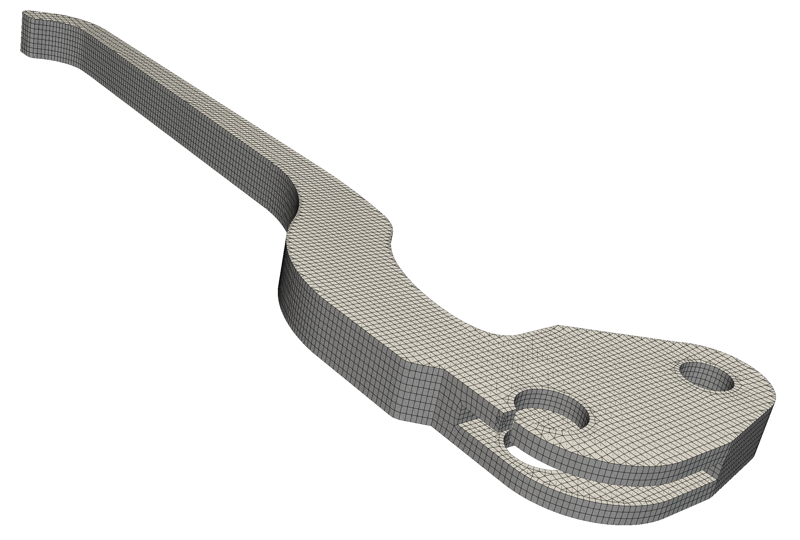
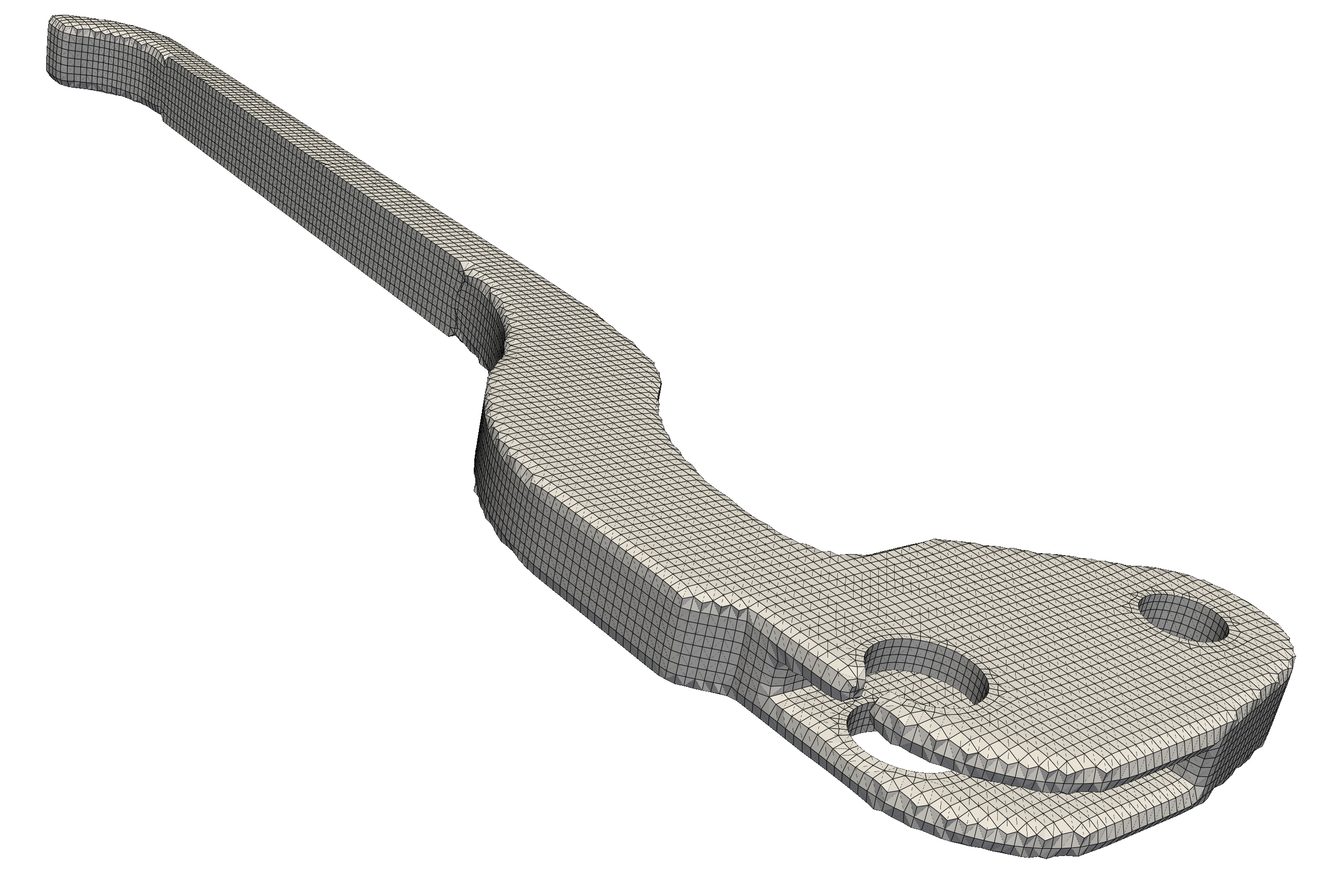
Mesh after using surfaceFeatureEdges utility to extract edges

The new mesh respects the geometry's sharp features much better. After a visual inspection, we should perform a formal quality check using the checkMesh utility:

checkMesh

From the output of checkMesh, we can see that the mesh passed the test and is OK for use:

...
Checking geometry...
        Overall domain bounding box (-0.0303905 -0.0243743 -0.00450006)
        (0.0203966 0.16956 0.00450007)
        Mesh has 3 geometric (non-empty/wedge) directions (1 1 1)
        Mesh has 3 solution (non-empty) directions (1 1 1)
        Boundary openness (6.16467e-16 -3.41217e-17 1.354e-16) OK.
        Max cell openness = 3.17123e-16 OK.
        Max aspect ratio = 8.35448 OK.
        Minimum face area = 2.98537e-08. Maximum face area = 1.96001e-06.
        Face area magnitudes OK.
        Min volume = 4.77543e-12. Max volume = 1.29557e-09.
        Total volume = 2.41888e-05. Cell volumes OK.
        Mesh non-orthogonality Max: 52.2587 average: 9.14128
        Non-orthogonality check OK.
        Face pyramids OK.
        Max skewness = 1.21589 OK.
        Coupled point location match (average 0) OK.
Mesh OK.

From the checkMesh output, we obtain the maximum values of mesh quality metrics such as aspect ratio, skewness, and non-orthogonality. All of these metrics are important, but for segregated solvers with semi-implicit discretisation, non-orthogonality is particularly critical. High non-orthogonality reduces the implicitness of the discretisation, which in turn decreases robustness and solver efficiency. Therefore, it should be kept as low as possible.

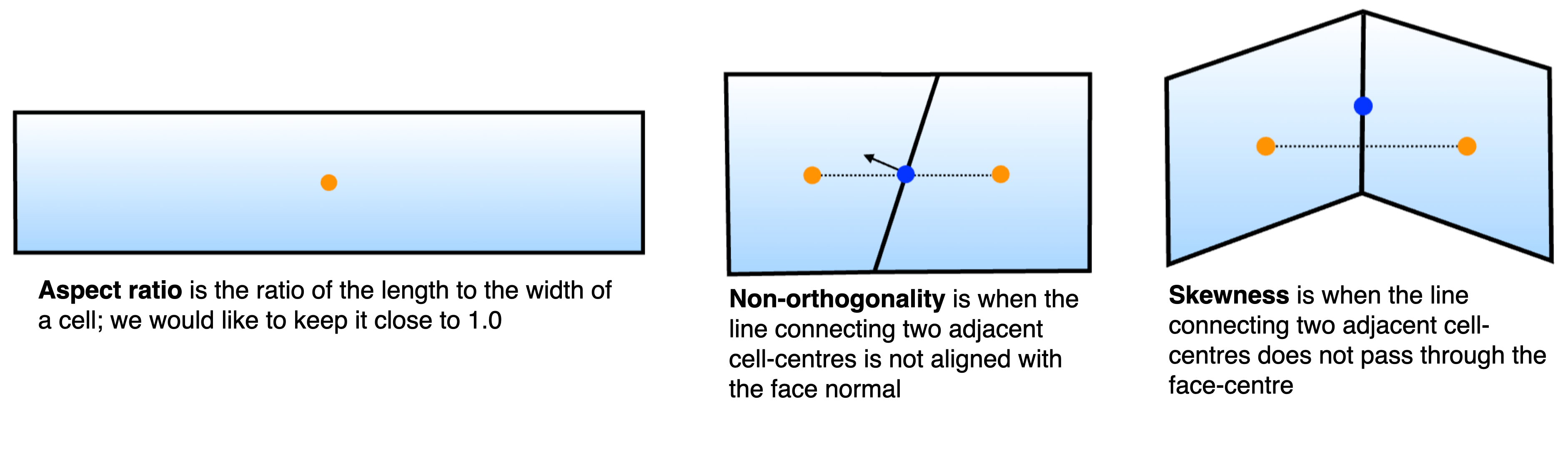
checkMesh mesh metrics explanation

The mesh is written in constant/polyMesh directory in OpenFOAM format, using files points, faces, owner, neighbour and boundary file. After generating the mesh , one should always inspect constant/polyMesh/boundary file. The mesher often assigns the default wall type to all patches. For applying traction and displacement boundary conditions, these must be changed to the generic patch type.

4
(
fixed
{
    type patch;
    nFaces 332;
    startFace 86415;
}
freeRotation
{
    type patch;
    nFaces 360;
    startFace 86747;
}
freeTraction
{
    type patch;
    nFaces 10340;
    startFace 87107;
}
load
{
    type patch;
    nFaces 624;
    startFace 97447;
}
)

Step 3. Preparing Case Files

With the mesh complete, we now need to configure the case files for the simulation.

Boundary and Initial Conditions

First, open the 0/D file to set the boundary and initial conditions for the displacement field D. We'll start with an initial condition of zero displacement for the entire domain:

internalField   uniform (0 0 0);

Next, we define the conditions for each boundary patch inside the boundaryField dictionary. The setup is as follows:

• fixed: Zero displacement is prescribed on this patch.
• freeRotation: This patch simulates a pin, allowing rotation but no surface normal movement. We use a boundary condition that enforces zero normal displacement and zero shear stress (tangential traction).
• freeTraction: This is a free surface with no applied forces.
• load: A pressure of 50 kPa is applied to this surface.

The final 0/D file should look like this:

boundaryField
{
    fixed
    {
        type            fixedDisplacement;
        value           uniform (0 0 0);
    }
    freeRotation
    {
        type            fixedDisplacementZeroShear;
        value           uniform (0 0 0);
    }
    freeTraction
    {
        type            solidTraction;
        traction        uniform ( 0 0 0 );
        pressure        uniform 0;
        value           uniform (0 0 0);
    }
    load
    {
        type            solidTraction;
        traction        uniform ( 0 0 0 );
        pressure        uniform 50000;
        value           uniform (0 0 0);
    }
}

Material and Solid Properties

Next, we need to adjust input dicts in the constant directory. Material properties are defined in constant/mechanicalProperties. We will specify the properties for aluminium:

planeStress     no;

mechanical
(
    aluminum
    {
        type            linearElastic;
        rho             rho [1 -3 0 0 0 0 0] 2700;
        E               E [1 -1 -2 0 0 0 0] 70+9;
        nu              nu [0 0 0 0 0 0 0] 0.33;
    }
);

In the constant/solidProperties file, we select the solid mechanics model and control the solver's behaviour. We will use the linearGeometryTotalDisplacement solver, which is a segregated solver for small strains and rotations.

// linearGeometry: assumes small strains and rotations
solidModel     linearGeometryTotalDisplacement;

"linearGeometryTotalDisplacementCoeffs"
{
    // Maximum number of momentum correctors
    nCorrectors     20000;

    // Solution tolerance for displacement
    solutionTolerance 1e-05;

    // Alternative solution tolerance for displacement
    alternativeTolerance 1e-05;

    // Material law solution tolerance
    materialTolerance 1e-05;

    // Write frequency for the residuals
    infoFrequency   100;
}

The other files in the constant directory (physicalProperties, dynamicMeshDict) can remain unchanged. The g file can be modified if you wish to include gravitational effects.

Numerical Schemes and Run-Time Control

The discretisation schemes in system/fvSchemes are mostly suitable, but it is important to ensure they are compatible with your OpenFOAM version. Different versions may use different names for gradient schemes (e.g., pointCellsLeastSquares). The solids4Foam::convertCaseFormat command, which we will add to the Allrun script later, automatically handles these updates.

In system/fvSolution, we can set solver settings and relaxation factors. Applying a small amount of under-relaxation to the displacement field D can improve stability in some cases without significantly affecting convergence speed.

solvers
{
    D
    {
        solver          PCG;
        preconditioner  FDIC;
        tolerance       1e-09;
        relTol          0.05;
    }
}

relaxationFactors
{
    equations
    {
        // D    0.999;
    }

    fields
    {
         D       0.99;
    }
}

Finally, in system/controlDict, we need to clean up the functions entry by removing forceDisp1 and plateHoleAnalyticalSolution1, which were copied from the tutorial case. We can also adjust the pointDisp function to monitor the displacement at a specific point on our brake lever. You will need to choose a coordinate that lies on the lever's geometry.

functions
{
    pointDisp
    {
        type          solidPointDisplacement;
        point         (-0.01 0.165 0);
    }
}

Step 4. Running the Case

We will run the case on multiple cores. The number of cores and decomposition method is set in system/decomposeParDict:

numberOfSubdomains 6;
method scotch;

To run the case, we will modify existing Allrun script. The script should look like this:

#!/bin/bash

# Source tutorial run functions
. $WM_PROJECT_DIR/bin/tools/RunFunctions

# Source solids4Foam scripts
source solids4FoamScripts.sh

# Check case version is correct
solids4Foam::convertCaseFormat .

# Run case in parallel
solids4Foam::runApplication decomposePar -cellDist
solids4Foam::runParallel solids4Foam
solids4Foam::runApplication reconstructPar

Make the script executable with the following command:

chmod +x Allrun

Now, you can run the entire simulation by simply executing the script:

./Allrun

To monitor residuals, we can open a new terminal and type the following command for live monitoring of the solver log file:

tail -f log.solids4Foam

Evolving solid solver
Solving the momentum equation for D
setCellDisplacements: reading cellDisplacements
    Corr, res, relRes, matRes, iters
    100, 0.0140041, 0.00915755, 0, 134
    200, 0.00660016, 0.00428296, 0, 146
    300, 0.00398494, 0.0029169, 0, 130
    400, 0.00329534, 0.0020852, 0, 137
    500, 0.00161131, 0.00166415, 0, 137
    600, 0.00148513, 0.00134746, 0, 138
    700, 0.00122678, 0.00107629, 0, 136
    800, 0.00143081, 0.000964108, 0, 139
    900, 0.000613834, 0.000810128, 0, 143
    1000, 0.000769182, 0.000691791, 0, 137
    1100, 0.000538599, 0.000636424, 0, 139
    1200, 0.000537587, 0.000558763, 0, 138
    1300, 0.000473058, 0.000502587, 0, 140
    1400, 0.000406682, 0.00044205, 0, 142
...

The solver log file is printing residuals as follows:

• res: This is residual of linear solver being used to solve system of equation.

• relRes: This is the relative residual, indicating the relative change in the solution between two successive iterations.

• matRes: This column, which is zero here, is only used for non-linear material models.

• iters: This is the number of iterations performed by the linear solver.

This case is dominated by bending, which presents a challenge for segregated solvers due to the strong coupling between displacement components. As a result, a higher number of outer correctors (nCorr) is required to reach convergence.

While the solver is running, you can inspect how the domain was decomposed by visualizing the cellDist field in ParaView. The field is generated using -cellDist flag when running decomposePar command.

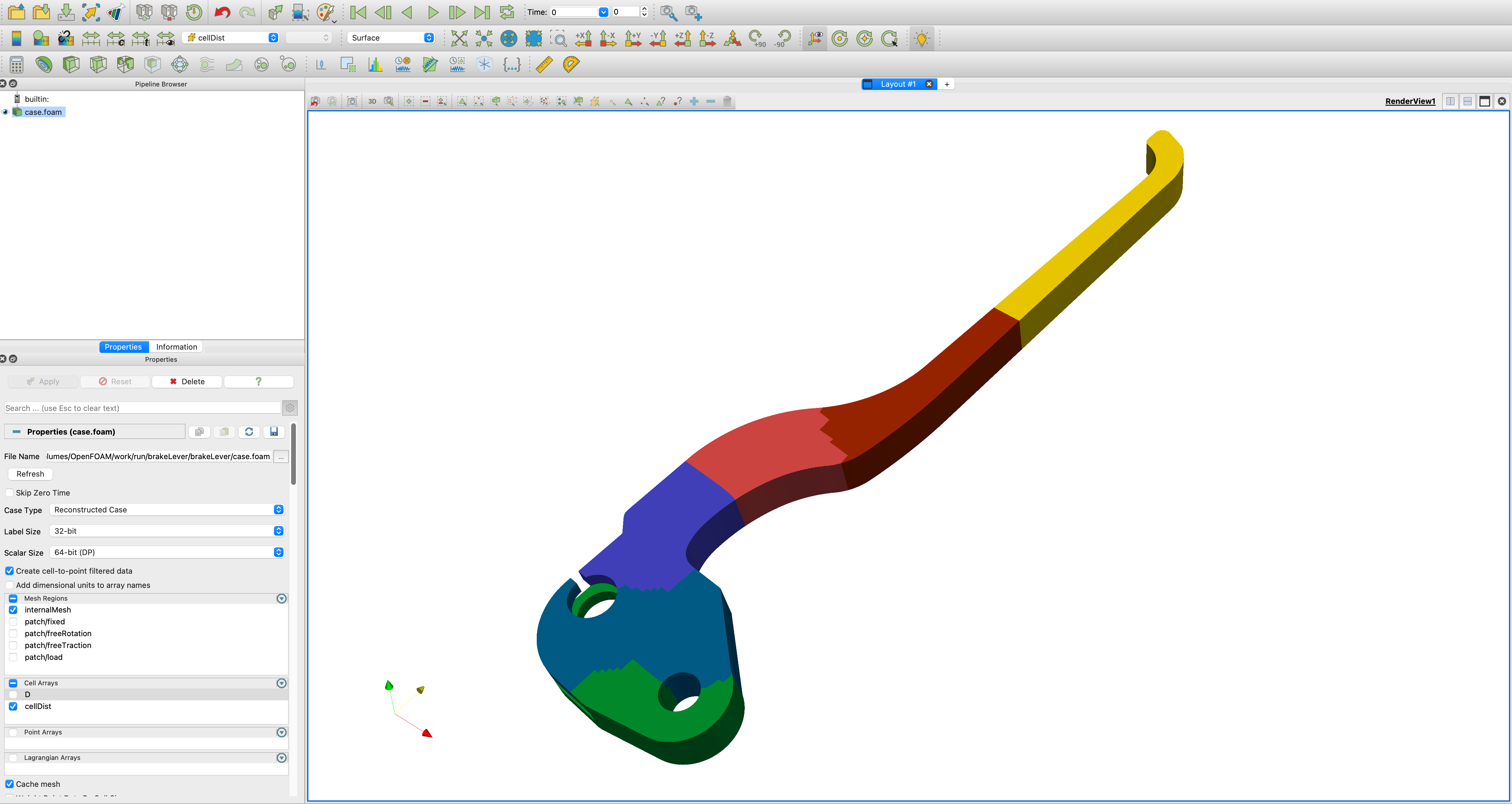
Computational domain decomposition, colours denote different processors

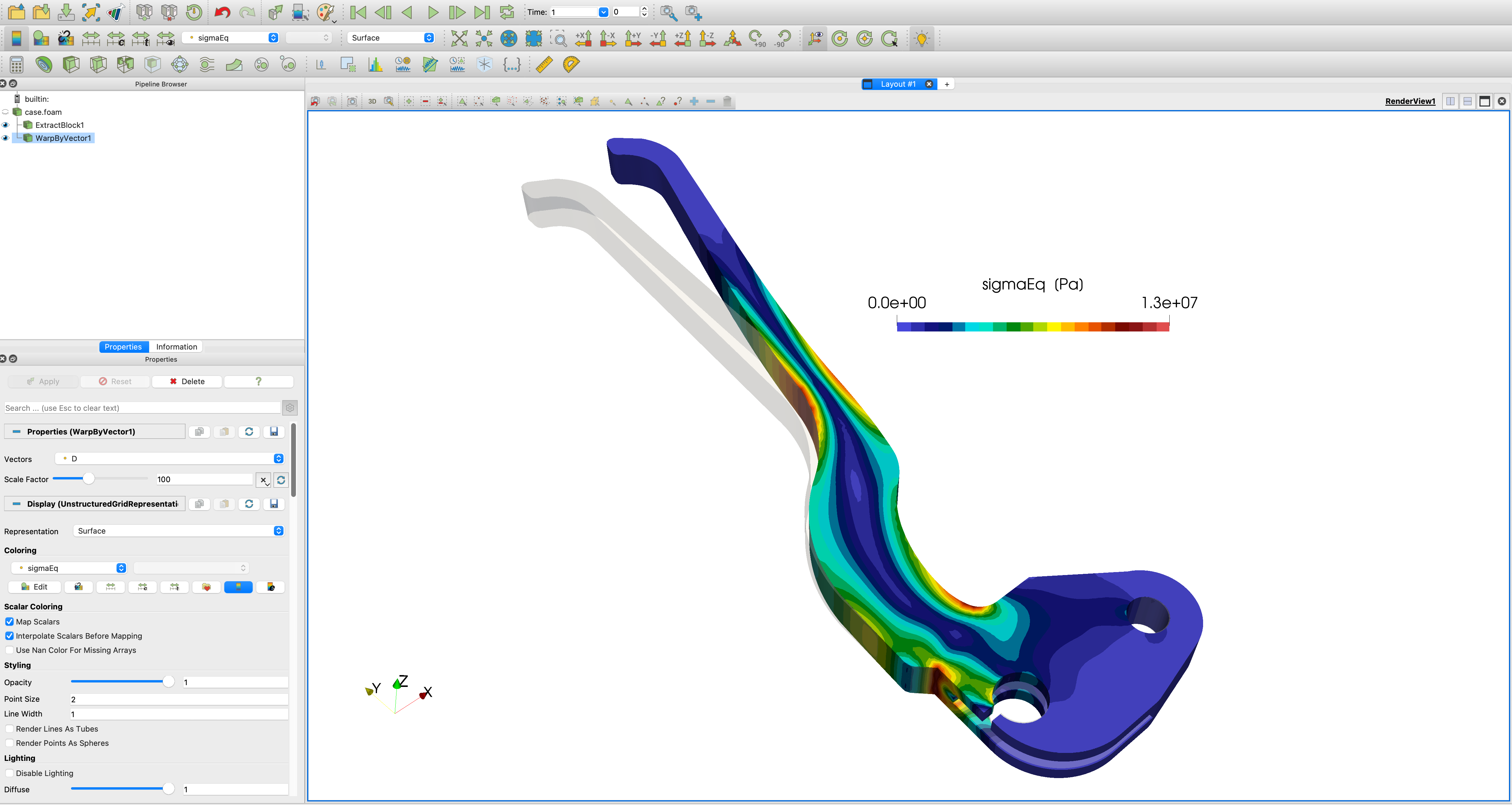
Step 5. Analysing the Results

Once the simulation is complete, open the results in ParaView:

paraview case.foam

When viewing the results in ParaView, we will warp the geometry by a scaled displacement field, which can be achieved using the Warp By Vector filter, where the D displacement field is selected as the Vector, and a Scale Factor of 1 shows the true deformation. In this case, using a Scale Factor of 100 allows the deformation to be seen. To compare the deformed shape with the original geometry, you can use the Filters > Alphabetical > Extract Block filter to create a separate object for the undeformed lever and then reduce its opacity. This allows you to see both the original and deformed states simultaneously.

Deformed geometry by resulting displacement (scaled by a factor of 100)