Free Flexible Beam: Kayak-Rowing Motion
Tutorial Aims
This tutorial demonstrates how to:
- simulate the strongly coupled three-dimensional motion of a free beam
- rotate a beam into a non-axis-aligned initial configuration
- apply time-dependent force and moment boundary conditions at a free end
- transition from forced motion to free vibration
- assess energy conservation with the Newmark time-integration scheme
The case is the third benchmark presented in the beamFoam paper.
Prerequisites
- A compiled beamFoam installation
- A sourced, supported OpenFOAM.com environment
- gnuplot with the
pdfcairoterminal for generating the supplied plots - ParaView for visualising the three-dimensional motion
The default case uses 10 beam segments, the Newmark scheme, deltaT = 0.01 s and an end time of 40 s.
Problem Description
An initially straight beam is inclined in the global xy-plane. Both ends are free, and a force and combined bending moment are applied at endpoint A, the right patch, until t = 2.5 s. The loads are then removed and the beam continues in free vibration.
The nonlinear interaction of bending in two planes with forward motion causes the free ends to trace paddle-like trajectories. This characteristic response is commonly called the kayak-rowing motion.
| Property | Value |
|---|---|
| Length | 10 m |
| Cross-section | circular |
| Radius | 0.44721360 m |
| Density | 1.5915466 kg/m^3 |
| Young's modulus | 1.5915494e4 Pa |
| Shear modulus | 1.5915494e4 Pa |
| Initial rotation | 53.130102 degrees about negative z |
Right-end force for 0 <= t <= 2.5 s | (8 0 0) N |
| Right-end moment magnitude | 80 Nm |
| Default mesh | 10 beam segments |
| Default time step | 0.01 s |
| End time | 40 s |
The selected cross-section and material properties correspond to:
EA = GA = 1e4 NEI = 500 Nm^2A rho = 1 kg/m- prescribed rotary inertia
I_2 rho = I_3 rho = 10 kg m
An artificial rotary-inertia scaling factor of 200.39427 is used to reproduce the benchmark inertia.
Case Setup
Beam Geometry and Initial Position
constant/beamProperties defines the circular beam, material properties and inertia scaling:
beamModel coupledTotalLagNewtonRaphsonBeam;

beams
(
    beam_0
    {
        crossSectionModel circle;

        circleCrossSectionModelDict
        {
            radius 0.44721360;
        }

        length      10;
        nSegments   10;
    }
);
After createBeamMesh, the Allrun script rotates the beam into its inclined initial configuration:
setInitialPositionBeam \
    -cellZone beam_0 \
    -translate '(0 0 0)' \
    -rotateAngle '((0 0 -1) 53.130102)'
Boundary Conditions and Loading
Both ends use Neumann boundary conditions:
0/WusesforceBeamDisplacementNRon theleftandrightpatches0/ThetausesmomentBeamRotationNRon theleftandrightpatches
Endpoint B, the left patch, has zero force and zero moment throughout the simulation.
Endpoint A, the right patch, receives:
- force
(8 0 0) N - moment
(56.568542495 56.568542495 0) Nm, with magnitude80 Nm
The loads remain active until t = 2.5 s and are removed between t = 2.5 s and t = 2.51 s. The time histories are stored in:
constant/timeVsForceLeftconstant/timeVsForceRightconstant/timeVsMomentLeftconstant/timeVsMomentRight
Time Integration and Output
system/fvSchemes selects the implicit Newmark method. The following function objects are enabled in system/controlDict:
beamDisplacements: displacement history at endpoint AbeamForcesMoments: force and moment history at endpoint BbeamConvergenceData: nonlinear convergence historybeamEnergyData: internal, kinetic and total energy histories
Running the Tutorial
From this tutorial directory:
./Allclean
./Allrun
The script performs:
createBeamMeshsetInitialPositionBeambeamFoamgnuplot allPlots.gnuplot
The main generated files are:
log.createBeamMeshlog.setInitialPositionBeamlog.beamFoamdisplacementPlot.pdfenergyPlot.pdfpostProcessing/0/beamDisplacements_right.datpostProcessing/0/beamEnergyData.dat
Post-Processing
To inspect the three-dimensional motion:
touch case.foam
paraview case.foam
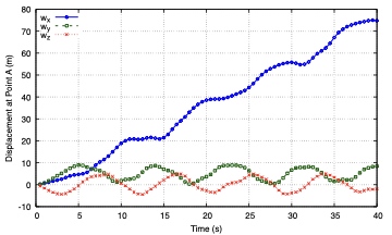
Apply Warp By Vector using pointW and animate the available time directories. Endpoint A should move forward in the x-direction while oscillating in y and z.
displacementPlot.pdf shows the three displacement components at endpoint A. energyPlot.pdf shows internal, kinetic and total energy.
Expected Results
The paper reports:
- negligible changes in the deformation pattern under mesh refinement
- approximately three Newton iterations per time step
- forward x-motion combined with y- and z-oscillation
- conservation of total energy after the loads are removed at
t = 2.5 swhen using Newmark - numerical energy decay when using backward Euler with
deltaT = 0.01 s
The total energy may change while the external loads perform work during the first 2.5 s. The energy-conservation assessment should therefore focus on the free-vibration interval after load removal.
Comparing Time-Integration Schemes
The default system/fvSchemes uses Newmark:
ddtSchemes
{
    default Newmark;
}

d2dt2Schemes
{
    default Newmark;
}
To investigate backward Euler, change both defaults to Euler, clean the case, and rerun it:
./Allclean
./Allrun
The backward Euler result should show stronger numerical damping. Restore Newmark before using this case as an energy-conservation benchmark.
Long-Duration Energy Test
The paper also investigates Newmark energy stability up to t = 1000 s using deltaT = 0.1 s and 0.01 s.
To reproduce a long-duration run:
- Set
endTime 1000insystem/controlDict. - Select the required
deltaT. - Increase
writeIntervalto avoid excessive field output. - Run
./Allcleanfollowed by./Allrun. - Inspect
postProcessing/0/beamEnergyData.dat.
The time-series files already define zero external loads through t = 1000 s.
Troubleshooting
- If the initial beam is not inclined, inspect
log.setInitialPositionBeam. - If endpoint A does not enter free vibration, check that the right-end force and moment histories drop to zero after
t = 2.5 s. - If total energy decays during the free-vibration interval, confirm that both time-derivative schemes use
Newmark. - If plotting fails, confirm that gnuplot supports the
pdfcairoterminal. The raw histories remain available underpostProcessing/.
References
- Bali, S., Taran, A., Tuković, Ž., Pakrashi, V., and Cardiff, P. (2025). beamFoam: A Cell-Centred Finite Volume Solver for Nonlinear Geometrically-Exact Beams in OpenFOAM. OpenFOAM Journal, 5, 180-210.
- Simo, J. C., and Vu-Quoc, L. (1988). On the Dynamics in Space of Rods Undergoing Large Motions: A Geometrically Exact Approach.
- Jelenić, G., and Crisfield, M. A. (1998). Geometrically Exact 3D Beam Theory: Implementation of a Strain-Invariant Finite Element for Arbitrary Nonlinear Behaviour.
- Boyer, F., et al. (2004). Geometrically Exact Beam Model for Slender Elastic Rods: Numerical Methods and Applications.