Decaying Taylor-Green vortex flow: decayingTaylorGreenVortex

Tutorial Aims

• Benchmarks the accuracy and order of accuracy of the newtonIcoFluid coupled Newton-Raphson fluid solver against the analytical solution for the decaying Taylor-Green vortex flow case.

Case Overview

The 2-D, transient Taylor–Green decaying vortex flow has an analytical solution for an incompressible laminar, viscous fluid ¹. Consequently, the case is well-suited for benchmarking the accuracy and order of accuracy (spatial and temporal) of a discretisation. The spatial domain is taken here as the unit square $[0, 1] \times [0, 1]$ m and the analytical solution in non-dimensional form is given by \(u(x, y, t) = e^{-2\pi^2 t/\text{Re}} \sin(\pi x) \cos(\pi y)\) \(v(x, y, t) = -e^{-2\pi^2 t/\text{Re}} \cos(\pi x) \sin(\pi y)\) \(p(x, y, t) = e^{-4\pi^2 t/\text{Re}} \frac{1}{4} \left[\cos(2\pi x) + \sin(2\pi y)\right] + C\)

where $u$ is the non-dimensional $x$ component of velocity, $v$ is the non-dimensional $y$ component of velocity, $p$ is the non-dimensional pressure, $t$ is time, $Re$ is the Reynolds number taken here to be $10$, and $C$ is an arbitrary constant.

The time-varying analytical solution for velocity is prescribed as a boundary condition using a custom boundary condition called decayingTaylorGreenVortexVelocity or a codedFixedValue boundary condition as follows:

    walls
    {
        //type            decayingTaylorGreenVortexVelocity;
        type            codedFixedValue;
        name            decayingTaylorGreenVortexVelocity;

        code
        #{
            const scalar Re = 10;
            const scalar t = db().time().value();
            const scalar pi = constant::mathematical::pi;
            const scalar A = Foam::exp(-2.0*sqr(pi)*t/Re);

            const scalarField x(patch().Cf().component(vector::X));
            const scalarField y(patch().Cf().component(vector::Y));

            const vectorField velocity
            (
                A*Foam::sin(pi*x)*Foam::cos(pi*y)*vector(1, 0, 0)
              - A*Foam::cos(pi*x)*Foam::sin(pi*y)*vector(0, 1, 0)
            );

            operator==(velocity);
        #};

        value           uniform (0 0 0);
    }

For pressure, a zero gradient condition is assumed: $\boldsymbol{n} \cdot \boldsymbol{\nabla} p = 0$. This condition is enforced through a custom condition called fixedGradientCorrected or the standard zeroGradient boundary condition. The fixedGradientCorrected condition applies boudnary non-orthogonal corrections, whereas zeroGradient does not. As noted above for the velocity field, boundary non-orthogonal corrections are required to achieve the theoretical order of accuracy on grids containing boundary non-orthogonality in the limited of mesh refinement.

As all pressure boundaries are of gradient type, the pressure field is defined up to a constant. To deal with this in the current case, the pressure in the cell closest to the centre of the domain is fixed to 0, although any cell could be chosen.

A utility called initialiseTaylorGreenVortex is provided in the case, which initialises the internal velocity and pressure fields to the analytical solution at $t = 0$ s. The initial velocity magnitude field is shown in Figure 1.

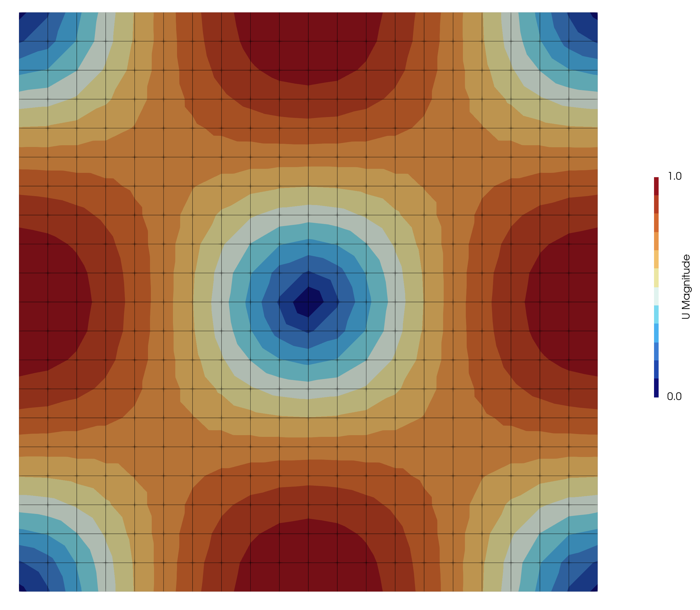
Figure 1: The velocity magnitude (in m/s) field at the initial time.

The case is examined using both static and moving meshes. Four variants of static mesh are consdered:

• Static 1: an orthogonal mesh, consisting of $N \times N$ quadrilateral cells constructed using blockMesh. To enable this mesh variant disable mesh all distortions by setting SMOOTHLYDISTORT=0 BUMP=0 PERTURB=0 in the configuration settings at the top of the Allrun script.

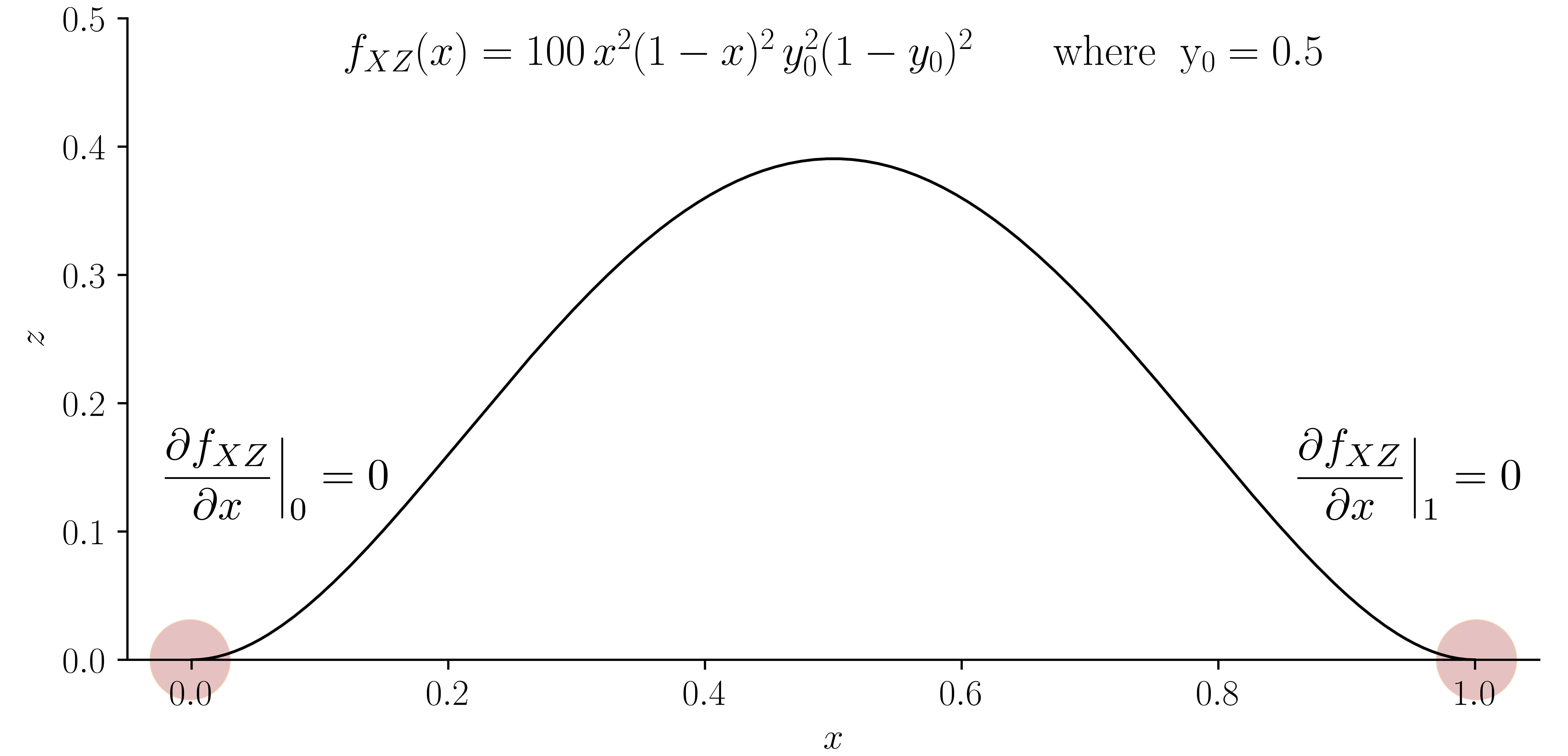
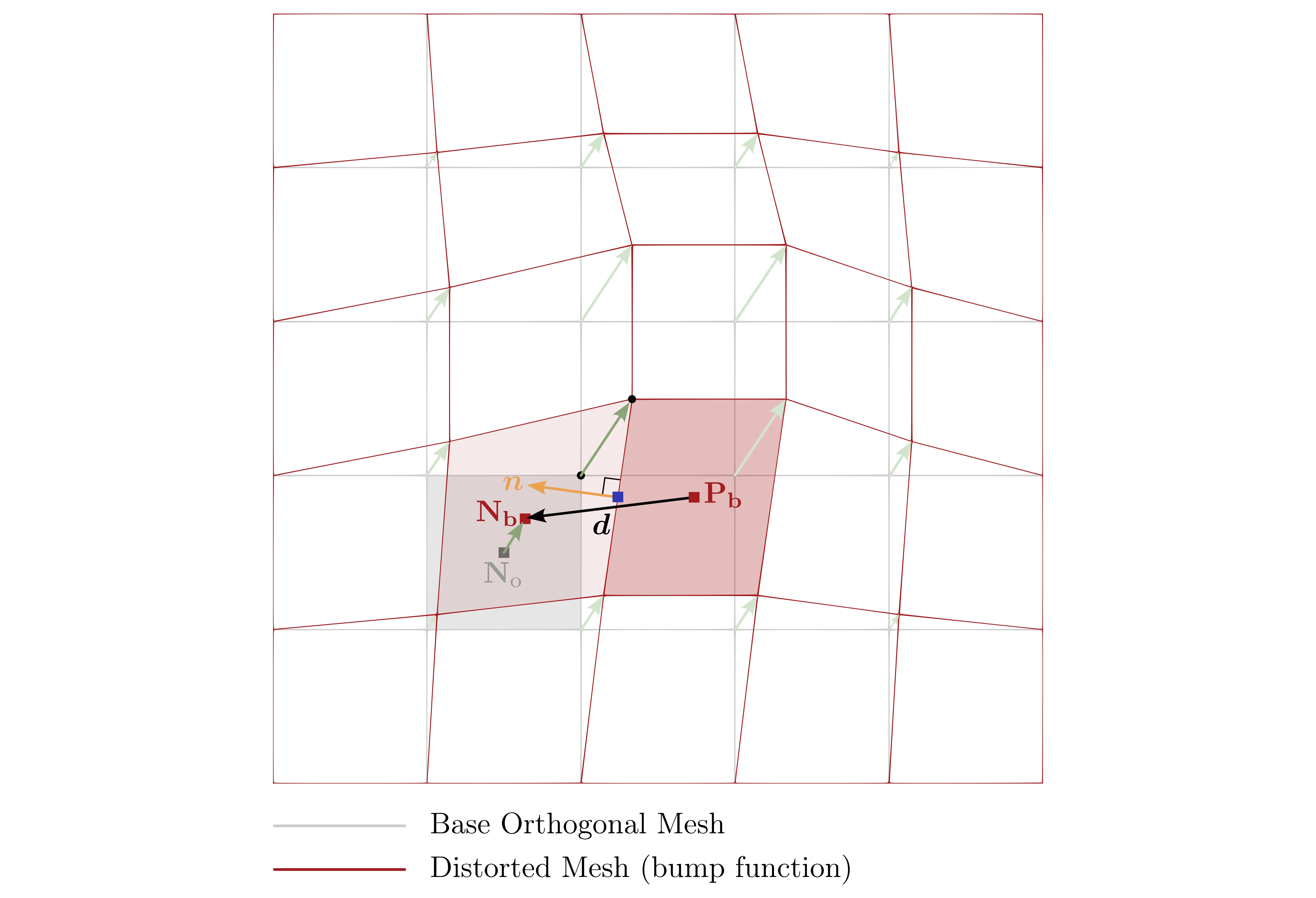
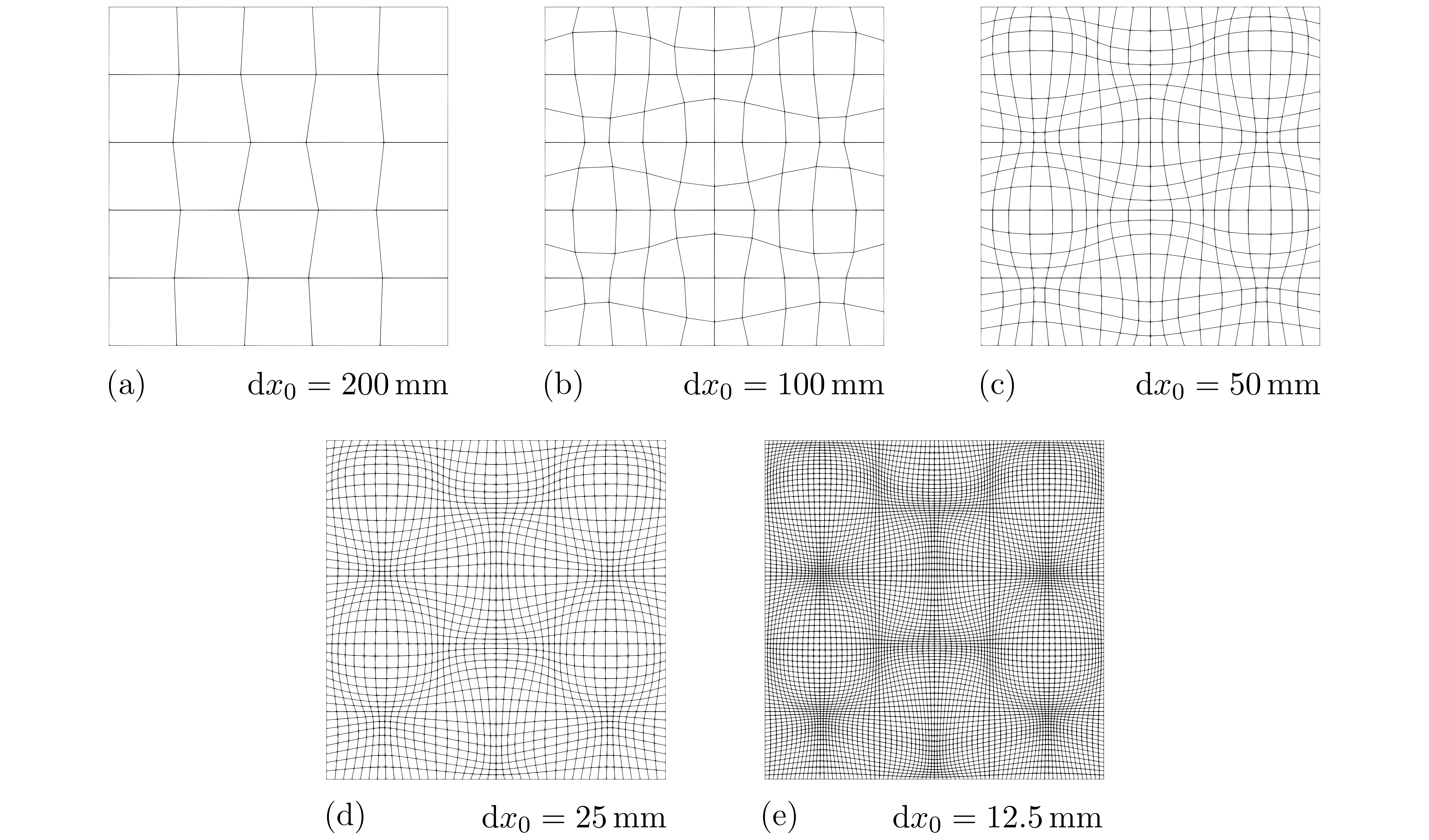
• Static 2: starts with the mesh from Static 1 and applies a smooth distortion to the internal mesh points using a bump function per below. This type of mesh can be generated by setting SMOOTHLYDISTORT=1 BUMP=1 PERTURB=0 in the configuration of the Allrun script. \(\mathbf{p}_i' = \mathbf{p}_i + \begin{bmatrix} A_x \\ A_y \\ A_z \end{bmatrix} f(x, y),\) \(f(x, y) = x^2(1 - x)^2 \, y^2(1 - y)^2.\)

• $\mathbf{p}_i$: original position of point $i$ in the orthogonal mesh
• $\mathbf{p}_i'$: new position of point $i$ after distortion

• $\mathbf{A} = (A_x, A_y, A_z)$: magnitude/scale vector

  

  

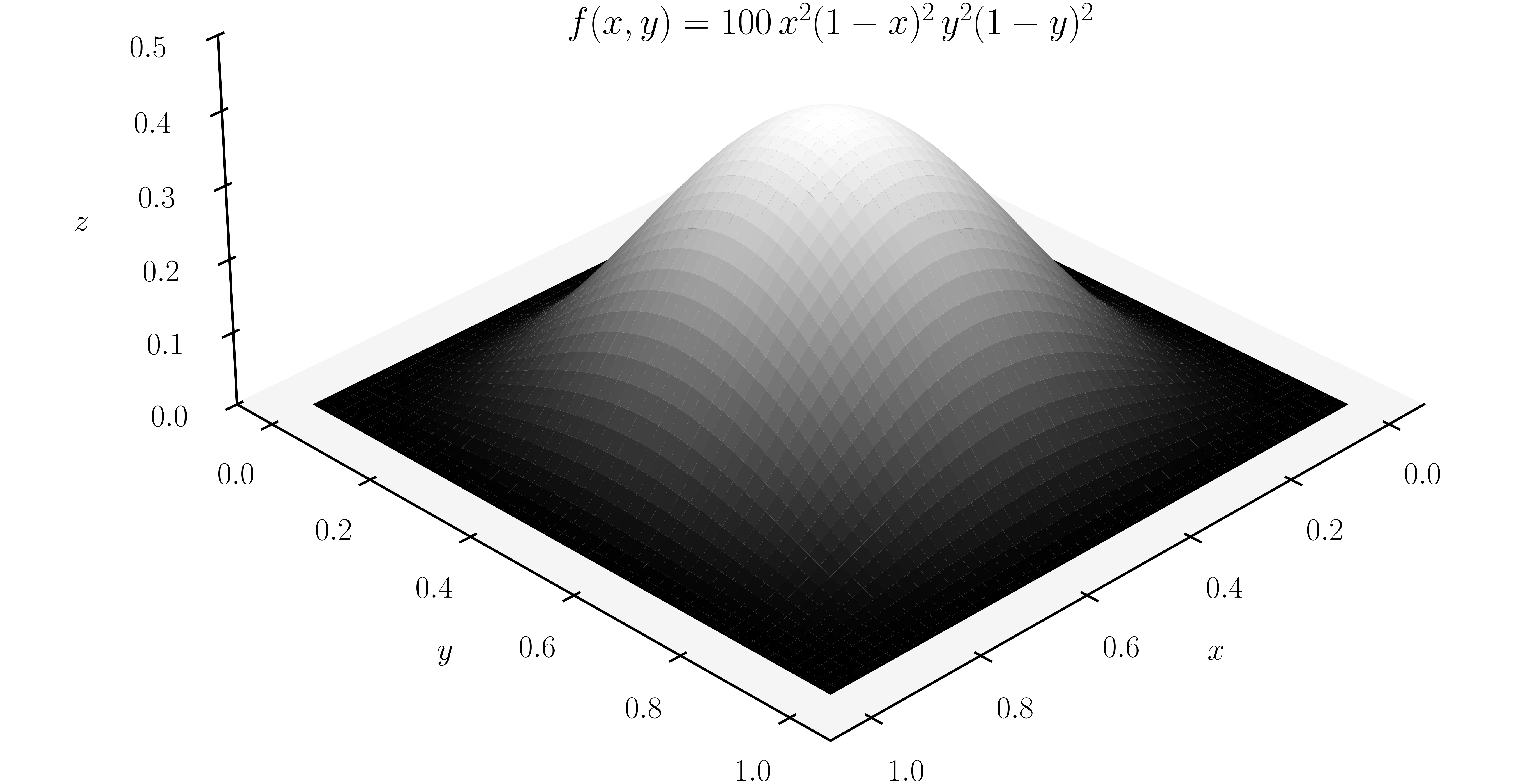
  As can be seen from the plots, the value of the function $f$ increases as we go toward the middle of the domain in the $x-y$ plane. This trend is also evident when comparing the distorted mesh with the original orthogonal mesh.

  

  Since the derivative of the bump function is zero at the domain boundary, the local face non-orthogonality goes to zero in the limit of mesh refinement; that is, the entire mesh becomes effectively orthogonal for fine meshes.

  

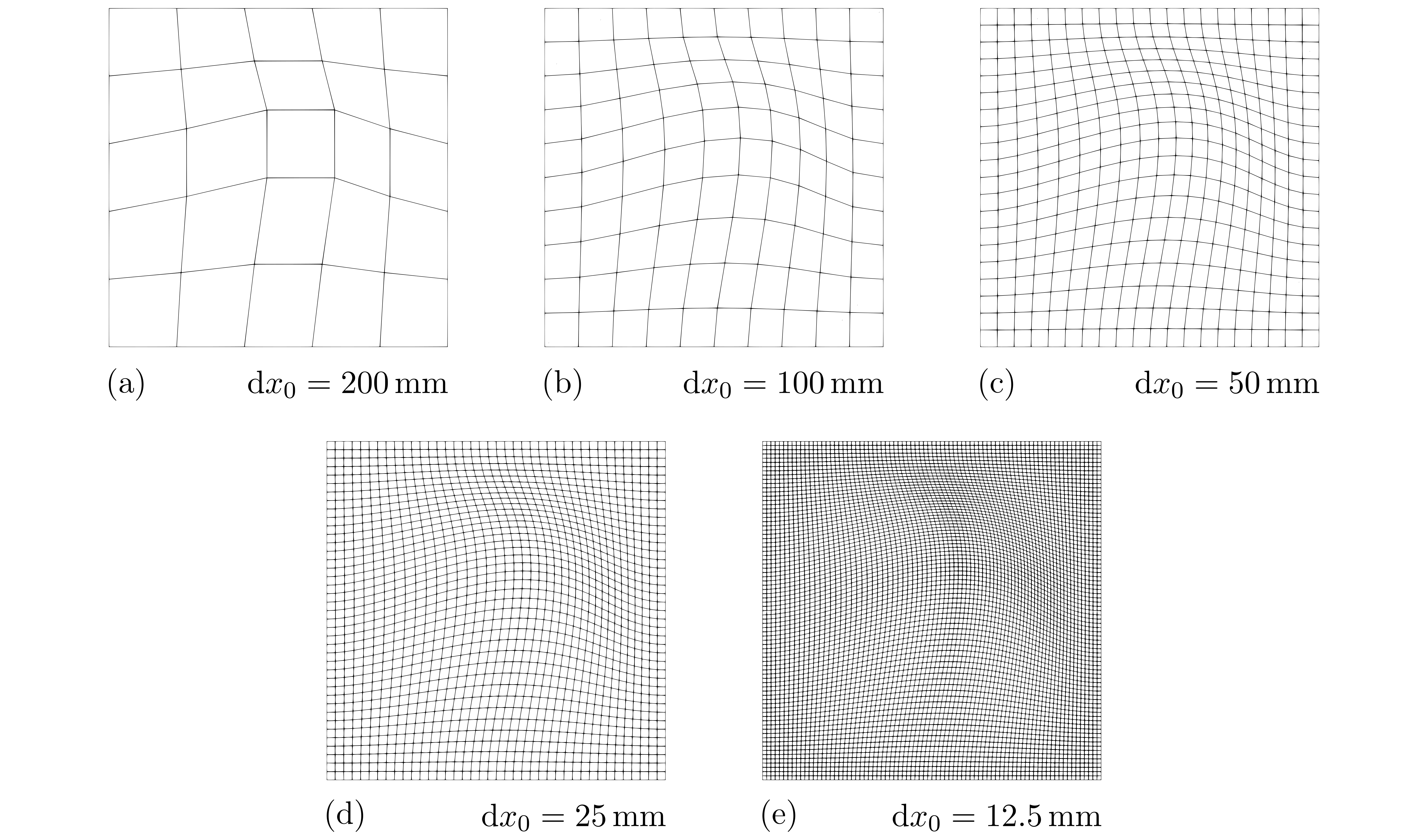
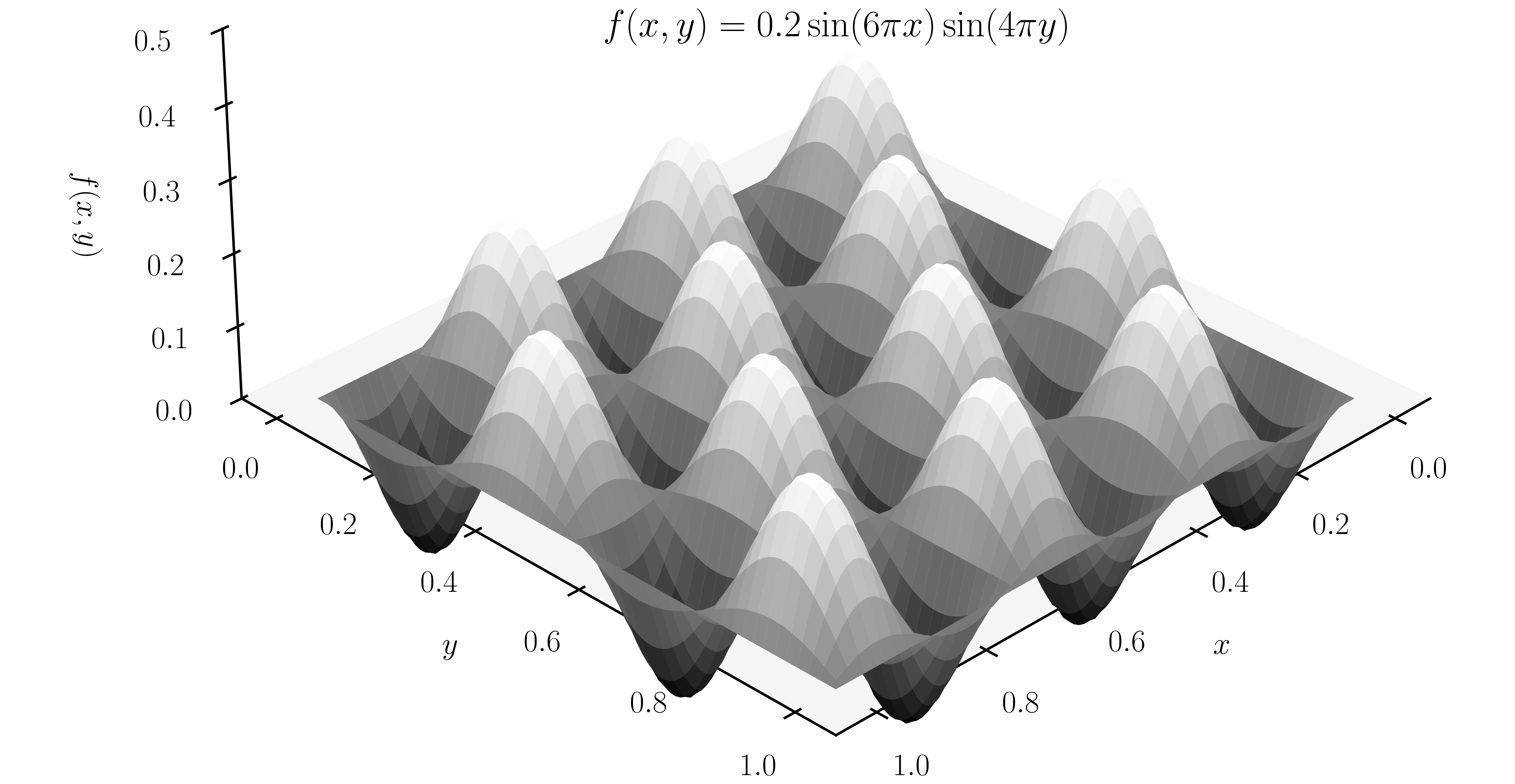
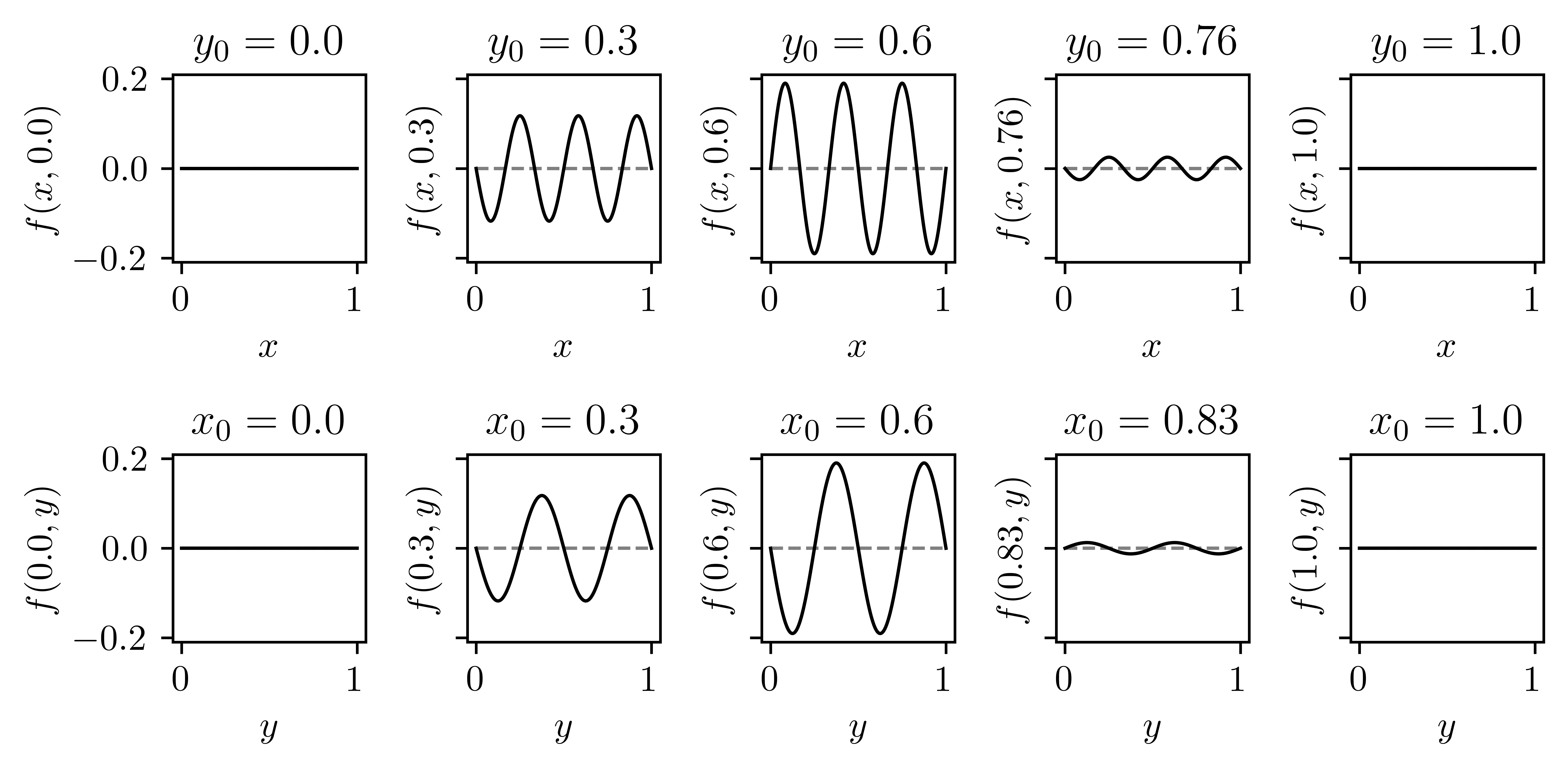
• Static 3: starts with the mesh from Static 1 and applies a smooth distortion to the internal points using a sinuisoidal function. This type of mesh can be generated by setting SMOOTHLYDISTORT=1 BUMP=0 PERTURB=0 in the configuration in Allrun. \(\mathbf{p}_i' = \mathbf{p}_i + \begin{bmatrix} f_x(x, y) \\ f_y(x, y) \\ f_z(x, y) \end{bmatrix},\) \(f_j(x, y) = A_j \sin(B_j \pi x) \sin(C_j \pi y) \quad \text{where}\quad j = x, y, z\)

• $\mathbf{p}_i$: original position of point $i$ in the orthogonal mesh
• $\mathbf{p}_i'$: new position of point $i$ after distortion
• $\mathbf{A} = (A_x, A_y, A_z)$: magnitude/scale vector

• $\mathbf{B} = (B_x, B_y, B_z)$ and $\mathbf{C} = (C_x, C_y, C_z)$: frequency vectors

  

  Like Static 2, the internal mesh faces become orthogonal in the limit of mesh refinement; however, unlike Static 2, finite non-orthogonality remains at the boundary faces even in the limit of mesh refinement.

  

  This is due to the fact that partial derivatives of the function are in general non-zero at the boundary.

  

  In this way, this variant assesses whether the discretisation consistently deals with boundary non-orthogonality.

• Static 4: starts with the mesh from Static 1 and applies a random perturbation to each internal mesh point. This type of mesh can be generated by setting SMOOTHLYDISTORT=0 BUMP=0 PERTURB=1 in the configuration in Allrun. The perturbation of a point is calculated as a scale factor times the local minimum edge length.

  \[\mathbf{p}_i' = \mathbf{p}_i + \begin{bmatrix} \text{rand}_x s_x l_i \\ \text{rand}_y s_y l_i \\ \text{rand}_z s_z l_i \end{bmatrix}\]
• $\mathbf{p}_i$: original position of point $i$ in the orthogonal mesh
• $\mathbf{p}_i'$: new position of point $i$ after perturbation
• $l_i$: local minimum edge length at point $i$
• $\text{rand}_x, \text{rand}_y, \text{rand}_z$: random numbers generated in $x$, $y$, and $z$ direction

• $\mathbf{s} = (s_x, s_y, s_z)$: scale factor vector

  Two types of distribution can be chosen:

  1. Gaussian Distribution: $\mathcal{N}(0, 1)$ (mean 0, variance 1)
  2. Uniform Distribution: $\text{Uniform}(-1, 1)$

  This perturbation is applied independently to each mesh level. Unlike previous variants, face non-orthogonality remains finite internally and at the boundary in this variant. As such, this variant is the most challenge static mesh from the discretisation perspective.

  

  Assessing the order of accuracy on these types of grids may require multiple simulations at each grid level using different random perturbation parameters; a best fit approach can then be used to determine the order of accuracy from the error vs average mesh spacing plots.

In addition to the static mesh variants, four moving mesh variants are considered:

• Moving 1: starting with the mesh from Static 1, a time-varying mesh motion is prescribed. The mesh is moved such that all mesh faces remain orthogonal. This allows the effect of mesh motion to be assessed independently of mesh non-orthogonality and skewness.
• Moving 2: the smooth mesh distortion from Static 2 is applied as a time-varying mesh motion. Like Static 2, internal and boundary face non-orthogonality go to zero in the limit of mesh refinement.
• Moving 3: the smooth mesh distortion of Static 3 is applied as a time-varying mesh motion. Like Static 3, internal face non-orthogonality go to zero in the limit of mesh refinement but boundary face non-orthogonality remains finite.

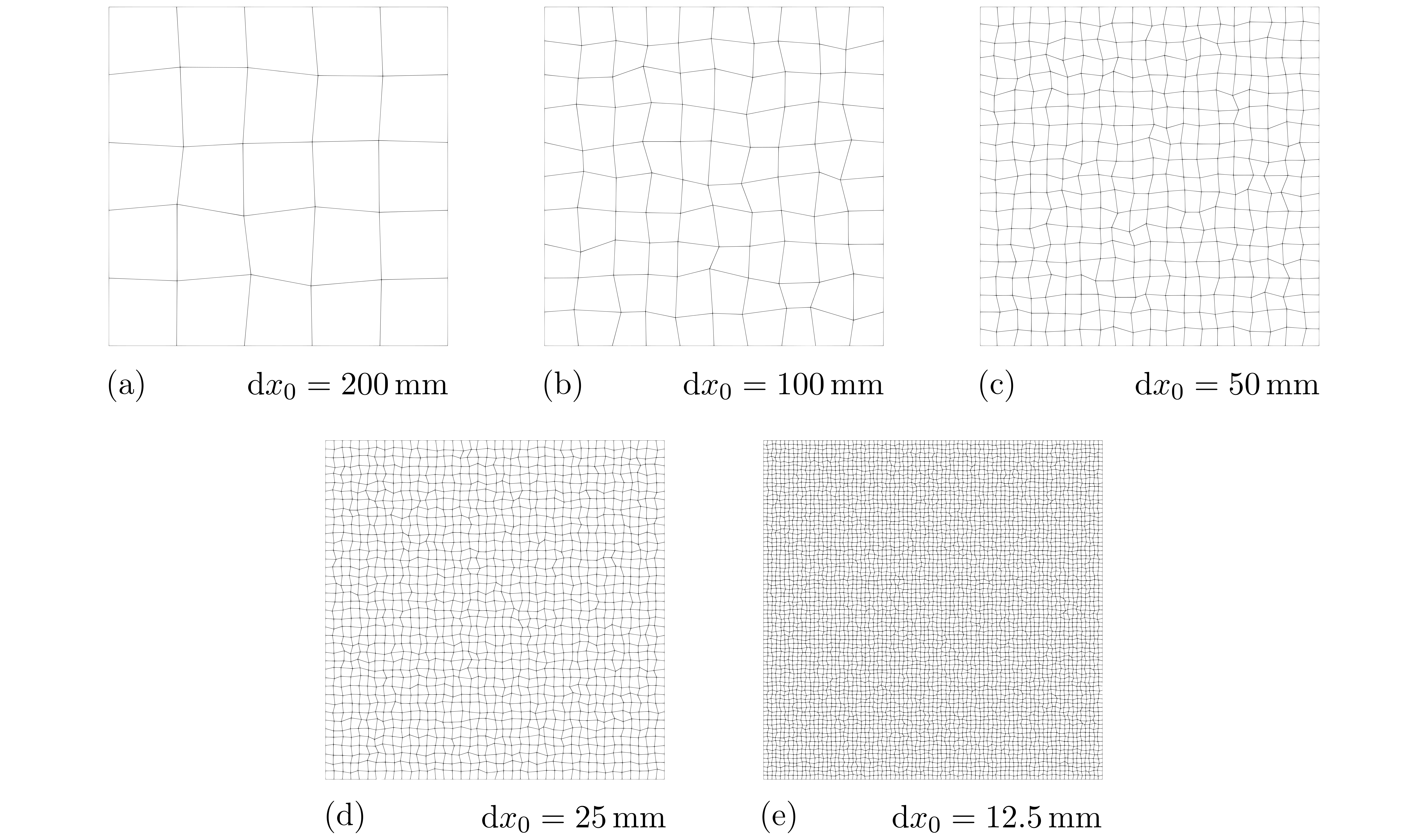
The base case contains multiple blockMeshDict files of increasing mesh density, which can be selected with the -dict option, e.g. blockMesh -dict system/blockMeshDict.uniform.3. The system/blockMeshDict.uniform.1 dictionary defines a mesh with $5 \times 5$ cells, and the number of cells in each direction is double for subsequent grids, e.g., system/blockMeshDict.uniform.2 contains $10 \times 10$ cells. The *.graded.* versions of the blockMeshDict dictionaries (e.g., system/blockMeshDict.graded.2) contain the same number of cells as the *.uniform.* versions, but apply mesh grading towards the walls, i.e. the cells are smaller near the walls and larger near the domain centre.

The case contains a function object, which calculates the exact velocity field exactU and the error norm in the velocity field ($L_1$, $L_2$, and $L_\infty$) at $t = 0.4$ s, as defined at the bottom of system/controlDict:

functions
{
    error
    {
        name    error;
        type    coded;
        libs    (utilityFunctionObjects);

        codeEnd
        #{
            // Define the exact U
            const scalar Re = 10;
            const scalar t = time().value();
            const scalar pi = constant::mathematical::pi;
            const scalar A = Foam::exp(-2.0*sqr(pi)*t/Re);

            volVectorField exactU
            (
                IOobject
                (
                    "exactU",
                    time().timeName(),
                    mesh(),
                    IOobject::NO_READ,
                    IOobject::AUTO_WRITE
                ),
                mesh(),
                dimensionedVector(dimVelocity, Zero)
            );

            {
                const scalarField x(mesh().C().component(vector::X));
                const scalarField y(mesh().C().component(vector::Y));

                exactU.primitiveFieldRef() =
                    A*Foam::sin(pi*x)*Foam::cos(pi*y)*vector(1, 0, 0)
                  - A*Foam::cos(pi*x)*Foam::sin(pi*y)*vector(0, 1, 0);
            }

            forAll(exactU.boundaryField(), patchI)
            {
                if (exactU.boundaryField()[patchI].size())
                {
                    const scalarField x
                    (
                        mesh().C().boundaryField()[patchI].component(vector::X)
                    );
                    const scalarField y
                    (
                        mesh().C().boundaryField()[patchI].component(vector::Y)
                    );

                    exactU.boundaryFieldRef()[patchI] =
                        A*Foam::sin(pi*x)*Foam::cos(pi*y)*vector(1, 0, 0)
                      - A*Foam::cos(pi*x)*Foam::sin(pi*y)*vector(0, 1, 0);
                }
            }

            exactU.correctBoundaryConditions();

            Info<< "Writing exactU to " << time().timeName() << endl;
            exactU.write();

            // Lookup U
            const auto& U = mesh().lookupObject<volVectorField>("U");

            // Calculate the error
            const volScalarField magError("magError", mag(U - exactU));
            Info<< "Writing magError to " << time().timeName() << endl;
            magError.write();
            const scalarField& Vol = mesh().V().field();
            const scalar totalVol = gSum(Vol);
            const vectorField diff(U - exactU);

            // Arithmetic errors
            // const scalar errorL1 = gAverage(mag(diff));
            // const scalar errorL2 = sqrt(gAverage(magSqr(diff)));
            // const scalar errorLInf = gMax(mag(diff));

            // Volume-weighted errors
            const scalar errorL1 = gSum(mag(diff*Vol))/totalVol;
            const scalar errorL2 = sqrt(gSum(magSqr(diff)*Vol)/totalVol);
            const scalar errorLInf = gMax(mag(diff));

            Info<< "Velocity errors norms:" << nl
                << "    mean L1 = " << errorL1 << nl
                << "    mean L2 = " << errorL2 << nl
                << "    LInf = " << errorLInf << endl;
        #};
    }
}

In this case, the newtonIcoFluid fluid solver is used, which solves the incompressible Navier-Stokes equations using a Jacobian-free Newton-Krylov approach ² built on the PETSc SNES nonlinear solver. The newtonIcoFluid settings are defined in constant/fluidProperties, where three types of settings are given: (i) numerical smoothing parameter for quelling checkerboarding oscillations, (ii) pressure reference point, and (iii) the PETSc options file, where the PETSc SNES nonlinear solver settings are defined.

fluidModel newtonIcoFluid;

newtonIcoFluidCoeffs
{
    // Smoothing terms
    // Trottenberg gives 1/16 for Stokes flow
    omega     [0 -2 1 0 0 0 0] 0.0625;
    localReRef 1e6;
    omegaExponent 1.0;
    alphaU    1.0;

    // Set the pressure to zero at the centre cell
    pRefPoint (0.5 0.5 0);
    pRefValue 0.0;

    // PETSc options file used by PETSc SNES
    optionsFile petscOptions.lu;
}

The petscOptions.lu file currently specifies a Jacobian-free Newton-Krylov solution approach, where the approximate Jacobian is inverted using a direct LU solver and L-GMRES is used as the iterative linear solver. Key settings from petscOptions.lu are shown below:

-snes_type newtonls
-snes_linesearch_type l2
-snes_max_it 1000
-snes_monitor
-snes_converged_reason
-snes_mf
-snes_mf_operator
-ksp_type lgmres
-ksp_gmres_restart 400
-ksp_converged_reason
-ksp_max_it 400
-pc_type bjacobi
-sub_pc_type lu

Running the Case

The case can be run using the included Allrun script located in the template case (decayingTaylorGreenVortex/base) directory or by executing the Allrun script in the parent decayingTaylorGreenVortex directory. The decayingTaylorGreenVortex/Allrun script runs multiple cases based on the configurations and mesh indices given at the top of the script, e.g.

configs=(
    "BASE=base NAME=hex.lu GRADED=1 \
    MOVING=0 ORTHOGONAL=0 \
    SMOOTHLYDISTORT=1 PERTURB=0 BUMP=0 \
    PIMPLEFOAM=1"
)

# ...

START_MESH=1
END_MESH=5

The decayingTaylorGreenVortex/Allrun script essentially performs five steps for each case configuration, in addition to perturbing the mesh, extracting results and generating plots:

# Build the utility for initialising the solution
wmake initialiseTaylorGreenVortex

# Copy 0.orig to 0
restore0Dir

# Create the mesh
runApplication blockMesh

# Initialise the velocity and pressure initial fields with the analytical
# solutions
runApplication initialiseTaylorGreenVortex

# Run the solver
runApplication solids4Foam

Expected Results

According to the analytical solutions given above, the magnitude of the velocity and pressure decrease in time, resulting the decay of the vortex. An animation of the velocity magnitude from $t = 0$ s to $t = 0.4$ s is shown in Video 1. The velocity streamlines, shown in black, are seen to remain stationary as the direction of the velocity field remains unchanged in time; instead, only its magnitude decreases.

Video 1: Evolution of the velocity magnitude field

The function object described above prints out the velocity field error norms at the end of the run after the last time step finished:

...

Time = 0.4

Evolving fluid model: newtonIcoFluid
Solving the fluid for U and p
  0 SNES Function norm 4.822871490313e-03
    Linear solve converged due to CONVERGED_RTOL iterations 2
  1 SNES Function norm 6.547206455521e-09
    Linear solve converged due to CONVERGED_RTOL iterations 2
  2 SNES Function norm 3.778722236831e-14
  Nonlinear solve converged due to CONVERGED_FNORM_RELATIVE iterations 2
ExecutionTime = 4.12 s  ClockTime = 5 s

Writing exactU to 0.4
Velocity errors norms:
    mean L1 = 0.000910565
    mean L2 = 0.000957898
    LInf = 0.00140902

End

Re-running the case for different mesh densities allows the order of accuracy of the solver to be assessed. Below the errors are given for five mesh spacings, where a spacing of $0.05$ m corresponds to the $20 \times 20$ grid described above ($1$ m divided into $20$ gives $0.05$ m).

# dx L1 L2 LInf
0.2 0.0128716 0.013683 0.0185237
0.1 0.00352244 0.00372265 0.00551404
0.05 0.000910565 0.000957898 0.00140902
0.025 0.000232169 0.000243816 0.000352236
0.0125 5.86993e-05 6.15957e-05 8.84018e-05

Plotting these errors on a log-log plot demonstrates that second-order is achieved as expected (Figure 2), where the $L_\infty$ (maximum) errors are larger than the $L_1$ and $L_2$ (average) errors, which is also as expected.

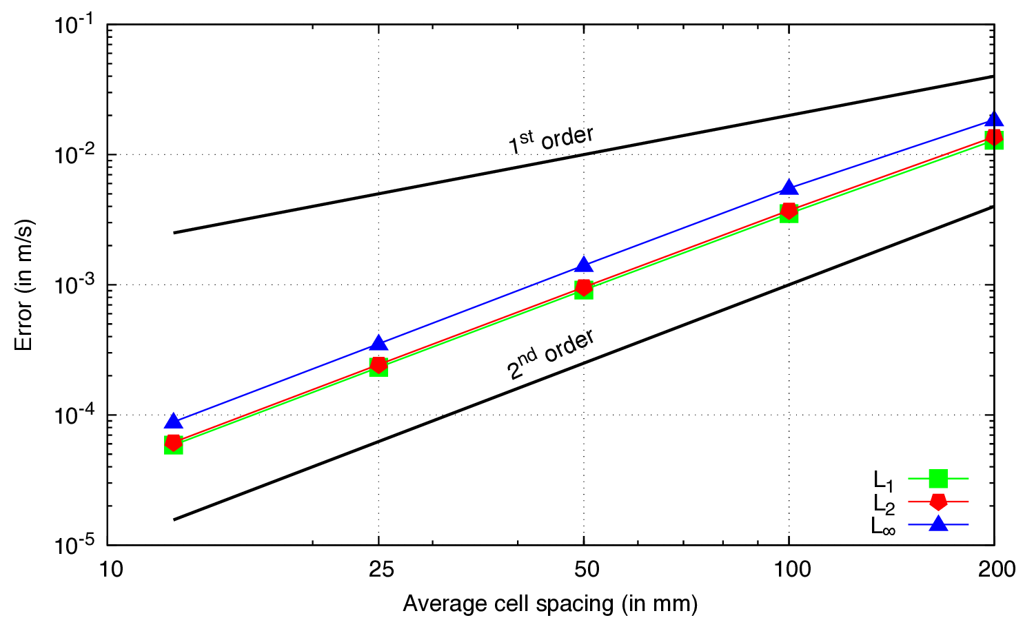
Figure 2: The velocity error norms as a function of mesh spacing.

References

Lagrangian–Eulerian formulation for solving moving boundary problems with large displacement and rotations, Journal of Computational Physics 255, 660–679](https://doi.org/10.1016/j.jcp.2013.08.038)

Implementing a Jacobian-free Newton-Krylov method in OpenFOAM Applications to solids fluids and fluid-solid interaction, 20th OpenFOAM Workshop, Vienna, Austria. July 2025](https://doi.org/10.13140/RG.2.2.35692.48009)